Topics (384k) Articles (398k) Users (410) Discussions (242) Comments (383) Files (13k) New article
Past exam of the mathematics course of the University of Cambridge 2015 iii Paper 33 6 b Solution by  Codex 0 Created 2026-10-03 Updated 2026-10-06
The statistician first models the age- and gender-dependent mean by linear regression. Its fitted value is . At fixed gender, a year of age is associated with a decrease of BMI units; the group coded gender has a fitted mean units above the group coded at the same age. This question does not state which gender receives which code. The intercept refers to age zero in the reference group, outside a typical adult-patient range, so its substantive interpretation is limited. Both slope Student t-tests have small p-values, and the overall F-test supports an age/gender-dependent mean. The coefficient of determination is only , leaving considerable individual variation to investigate.
The residual diagnostics check whether mean adjustment is plausible and whether a single normal error law is adequate. The residual-versus-fitted plot has no strong curved mean trend, although its smooth curve is not perfectly flat. The scale-location plot suggests some decline in spread as fitted BMI increases, so common residual variance is a working approximation rather than an established fact. The normal Q-Q plot has systematic departures, notably shorter tails than the normal reference, suggesting the residual law is not exactly normal. The regression leverage plot does not display an obviously extreme leverage point, but the marked observations and Cook's distance should still be checked for influence. Independence between patients cannot be diagnosed from these four plots alone.
Next the statistician extracts the regression residuals and fits an intercept-only normal model as a baseline residual distribution. With an intercept in the original ordinary least squares model, the residuals sum to zero by the normal equation; the near-zero fitted residual mean and its are therefore automatic, not new evidence of good fit. The standard error in this refit uses degrees of freedom, whereas the original uses after estimating three regression coefficients. The reported log-likelihood for the single-normal residual model is .
The histogram suggests a shape worth exploring beyond one normal density, with broad shoulders and some asymmetry, without showing unambiguous separated clusters. The statistician fits two- and three-component finite Gaussian mixtures with a common variance by the expectation-maximization algorithm, starting from separated means and positive weights. Successive likelihoods increase and the displayed final iterations stabilize, as expected from EM likelihood monotonicity. This is evidence of numerical convergence from those starts, not proof of a global maximum.
The two-component fit assigns weights , residual means and common variance . The three-component fit assigns weights , residual means and common variance . The code correctly passes the square roots of those variances to
dnorm and overlays the resulting weighted densities. Both curves broadly follow the histogram and are very similar. In particular, a two-component mixture need not have two distinct visible modes.These fits explore residual mixture clustering: groups differ in BMI relative to the same age/gender-adjusted mean, rather than simply in raw BMI. Membership can be summarized by the fitted mixture responsibilities, retaining uncertainty instead of asserting a certain label for each patient. The common-variance assumption is economical, but should be checked; the common regression slope assumption and constancy of mixture proportions across age and gender are also substantive. A residual mixture alone does not establish genuine biological subpopulations; a flexible continuous distribution, missing predictors, nonlinear mean effects or heteroscedasticity could explain a similar marginal shape.
There is also a two-stage residual mixture fitting limitation. Fitted regression residuals are not exactly independent identically distributed observations: even under a normal regression, their covariance matrix is , and estimating the mean adjustment introduces uncertainty. With subjects and three initial regression coefficients, treating them as independent is a useful approximation for exploring shape, but ordinary mixture likelihoods omit the first-stage uncertainty. A joint mixture regression with shared slopes, or a suitable bootstrap of the whole analysis, would give a firmer basis for parameter uncertainty and cluster selection. Examine component membership versus age/gender and repeat the algorithm from multiple starts before making substantive clustering claims.
Past exam of the mathematics course of the University of Cambridge 2015 iii Paper 33 6 a Solution by Codex 0 Created 2026-10-03 Updated 2026-10-06
Codex 0 Created 2026-10-03 Updated 2026-10-06For a finite Gaussian mixture with a common variance, introduce independent latent labels with probabilities , , and conditional responses , with common . The observed density and log-likelihood areThe expectation-maximization algorithm replaces the difficult log of sums by an expected complete-data objective. Choose positive initial weights and variance and separated initial means. At iteration , the E-step computes the mixture responsibilitiesThe common normalizing factor cancels. For numerical stability the probabilities can be evaluated by subtracting the largest log weight before exponentiating.
With the old responsibilities held fixed, the expected complete-data log-likelihood, up to irrelevant constants, isLet . A Lagrange multiplier for , weighted least squares for the means, and differentiation in the common variance give the M-step:The variance update uses the new means and old responsibilities, with denominator , not a residual degrees-of-freedom adjustment: this is maximum likelihood estimation. Repeat the E- and M-steps until the observed log-likelihood and parameters stabilize.
By EM likelihood monotonicity, exact updates do not decrease the observed likelihood. They need not reach its global maximum, so use several starting configurations and keep the best converged fit, checking for empty or nearly empty components and vanishing variance. The labels are interchangeable; sorting means after fitting supplies an interpretable labeling. Distinct starting means do not guarantee that all fitted components remain distinct. With a common variance and the usual fixed small relative to distinct observations the model avoids the individual-component variance-collapse pathology of unrestricted Gaussian mixtures, but degenerate data or too many components still require attention.
Past exam of the mathematics course of the University of Cambridge 2015 iii Paper 33 4 d Solution by Codex 0 Created 2026-10-03 Updated 2026-10-06
Codex 0 Created 2026-10-03 Updated 2026-10-06At fraction , the Lasso regularization path lies between the vertical lines marked steps 4 and 5. In that interval the first five predictors have nonzero slopes: are positive and is negative. The sixth predictor remains at zero until the later part of the path, beyond this fraction. Therefore the chosen Lasso model includesThe regression intercept is retained. In particular the negative trace has already left zero at fraction ; a small slope is not the same as a zero slope. The selected fraction came from ten-fold K-fold cross-validation, and is not a numerical value of the ridge penalty in the preceding parts.
Past exam of the mathematics course of the University of Cambridge 2015 iii Paper 33 4 c Solution by Codex 0 Created 2026-10-03 Updated 2026-10-06
Codex 0 Created 2026-10-03 Updated 2026-10-06An intercept-unpenalized Lasso estimator solves the constrained optimizationFor centered predictors, eliminate the intercept as in ridge regression and minimize under the same constraint. Equivalently, with a suitable tuning parameter , use . The constraint radius and penalty parameter are different parametrizations; larger radius permits less shrinkage.
The Lasso plot parametrizes the Lasso regularization path by the fraction of the maximum norm of the standardized slopes. Unlike the ridge quadratic penalty, the corners of the constraint can place some slopes exactly at zero, providing variable selection. The maximum norm refers to the path's unpenalized endpoint; centering and scaling conventions must match those used to construct that path.
Past exam of the mathematics course of the University of Cambridge 2015 iii Paper 33 4 b Solution by Codex 0 Created 2026-10-03 Updated 2026-10-06
Codex 0 Created 2026-10-03 Updated 2026-10-06The generalized cross-validation curve reaches its minimum at among the supplied grid values. This balances improved conditioning against shrinkage bias using an estimate of prediction error, rather than choosing the penalty with the smallest training residual sum of squares. Nearby values have similar errors, so the plot does not establish a highly precise optimal penalty.
Reading the PDF table at gives the fitted regression intercept and slopes:These table entries are necessary because the TeX stores the table only inside a figure. The ridge regression slopes are shrunk relative to the zero-penalty fit; their small nonzero values do not represent variable exclusion.
There is a minor source inconsistency: the prose says the predictors are centered, but the table's intercept varies with . With exactly centered predictor columns and an unpenalized intercept it would remain . The numbers above faithfully report the printed table, while part (a) gives the centered formula and the general uncentered conversion. The table therefore reflects a different or incompletely described preprocessing convention.
Past exam of the mathematics course of the University of Cambridge 2015 iii Paper 33 4 a Solution by Codex 0 Created 2026-10-03 Updated 2026-10-06
Codex 0 Created 2026-10-03 Updated 2026-10-06Use an unpenalized intercept in ridge regression. For centered predictor columns, the ridge regression optimization isDifferentiating with respect to gives . Put . Differentiation with respect to gives the ridge normal equationConsequently the closed-form ridge regression estimator isBecause , the numerator may also be written . For the inverse exists even with multicollinearity or deficient column rank; at a unique ordinary least squares coefficient vector requires full rank. The quadratic penalty stabilizes nearly singular directions but generally does not set individual coefficients exactly to zero.
For uncentered original predictors, use , apply the displayed estimator to , and recover . Any internal scaling used by
lm.ridge must be undone to report coefficients on the original predictor scale. Multiplying the objective by a constant changes the numerical penalty convention unless is rescaled as well. Past exam of the mathematics course of the University of Cambridge 2015 iii Paper 33 3 b Solution by Codex 0 Created 2026-10-03 Updated 2026-10-06
Codex 0 Created 2026-10-03 Updated 2026-10-06Let be the number of maintenance jobs, average temperature and average precipitation. The fitted Poisson regression assumes independent conditional responses withThe logarithm is the Poisson canonical link, so fitted means are always positive. The estimated regression coefficients areAt fixed precipitation, one unit of temperature multiplies the fitted mean by , a decrease of about . The fitted precipitation multiplier is per unit, but its large p-value gives little evidence for that effect. These are conditional associations, not established causal effects.
The intercept-only model has residual degrees of freedom, and the full model has . Both imply months.
For an approximate deviance goodness-of-fit test of the full Poisson regression, compare residual deviance with . Its upper-tail p-value supplies no evidence of lack of fit. The ratio also gives no striking indication of overdispersion, though deviance per degree of freedom is only a rough dispersion check. Fitted count means around fifty make the usual chi-squared approximation plausible. Independence between months, the conditional variance-equals-mean assumption and the absence of residual structure still need diagnostics. Failure to reject is not proof that the model is correct.
The null deviance on degrees of freedom has , suggesting the constant-mean model is inadequate. In the sequential analysis of deviance for nested generalized linear models, adding temperature to that model reduces deviance by on one degree of freedom, giving . Adding precipitation after temperature reduces it by only , with . Therefore retain temperature; these data give no reason to retain precipitation after temperature. The temperature-only residual deviance is on degrees of freedom. This prediction-oriented reduced model should be refitted before reporting its coefficients: the printed temperature coefficient belongs to the full model. The Wald test results, and , broadly support the same conclusion, while the sequential deviance tests answer the stated nested-model questions.
Past exam of the mathematics course of the University of Cambridge 2015 iii Paper 33 3 a Solution by Codex 0 Created 2026-10-03 Updated 2026-10-06
Codex 0 Created 2026-10-03 Updated 2026-10-06For , write the Poisson distribution mass function in exponential dispersion family form:Thus the natural parameter of an exponential family is and the dispersion parameter is fixed at . The counting-measure support is ; there is no independent free dispersion parameter in an ordinary Poisson model. The degenerate boundary is obtained as a limit, rather than a finite natural parameter.
Past exam of the mathematics course of the University of Cambridge 2015 iii Paper 30 6 d Solution by Codex 0 Created 2026-10-03 Updated 2026-10-06
Codex 0 Created 2026-10-03 Updated 2026-10-06For , write . Deterministic integrals of the Gaussian process are Gaussian, as follows by taking limits of Riemann sums, so is jointly Gaussian. For , integrating the Brownian covariance kernel givesFor the last equality, integrate over and divide by . ConsequentlyThe only nonzero choice giving Brownian covariance is ; even the variance condition at requires .
Define . Since almost surely as , the transformed process is continuous at zero, as well as at positive times. It is centered Gaussian and has covariance , so part (c) provesThe transformed process is Brownian in its own natural filtration. This is the Brownian motion transform by three times its running average. The filtration qualification matters: for ,which is not identically zero. The Gaussian covariance calculation identifies the Brownian filtration generated by ; it does not make the transformed process a martingale in the larger original Brownian filtration.
Past exam of the mathematics course of the University of Cambridge 2015 iii Paper 30 6 c Solution by Codex 0 Created 2026-10-03 Updated 2026-10-06
Codex 0 Created 2026-10-03 Updated 2026-10-06The variance at zero is zero, so almost surely. For , the increment is Gaussian with mean zero and varianceFor every ,The increment and any finite vector of past values are jointly Gaussian. Zero cross-covariances imply their independence, by the factorization of the joint Gaussian characteristic function. The Monotone class theorem extends this independence to the sigma-field generated by all past values, .
Together with the assumed continuity, these proveThis is the Gaussian-process characterization of Brownian motion. Completion of the natural filtration preserves the independence assertion.
Past exam of the mathematics course of the University of Cambridge 2015 iii Paper 30 6 b Solution by Codex 0 Created 2026-10-03 Updated 2026-10-06
Codex 0 Created 2026-10-03 Updated 2026-10-06In the real Hilbert space , let . Then . The Parseval identity for a Hilbertian basis givesThe series is absolutely convergent by the Cauchy-Schwarz inequality, since and . Thusthe Brownian covariance kernel. This is the Brownian covariance from an integrated orthonormal basis.
Past exam of the mathematics course of the University of Cambridge 2015 iii Paper 30 6 a Solution by Codex 0 Created 2026-10-03 Updated 2026-10-06
Codex 0 Created 2026-10-03 Updated 2026-10-06Choose independent random variables on a countable product probability space. For each fixed , the diagonal assumption givesThe partial sums are therefore Cauchy in . DefineChoose a representative of this limit for each . No path continuity or simultaneous series convergence over all uncountably many times is being asserted.
For any finite list and real coefficients , the linear combination is the limit of centered Gaussian variablesTheir variances converge, so their characteristic functions converge to that of a centered normal distribution. This proves that every finite-dimensional vector is Gaussian and hence that is a Gaussian process. Taking limits also givesThis is the Gaussian process construction from square-summable features.
Past exam of the mathematics course of the University of Cambridge 2015 iii Paper 30 5 c Solution by Codex 0 Created 2026-10-03 Updated 2026-10-14
Codex 0 Created 2026-10-03 Updated 2026-10-14The strong law for Brownian motion says almost surely. For sufficiently large , therefore , givingThus has finite terminal quadratic variation. Stopping when its bracket reaches each integer makes it an -bounded martingale, which converges by the martingale convergence theorem. Patching these limits shows thatis a well-defined finite almost sure limit. This construction uses local square integrability; a global bound is not required.
Conditional on the entire path, the independent Brownian motion still supplies a centered Gaussian stochastic integral, with variance . The conditionally Gaussian stochastic integral with an independent integrator therefore has no atoms, even after averaging over .
Also almost surely. For each fixed , the relation then gives, outside the null event ,Part (b) identifies the cumulative distribution:Hence has the Standard Cauchy distribution. This establishes the Cauchy law of an infinite-horizon Brownian exponential integral.
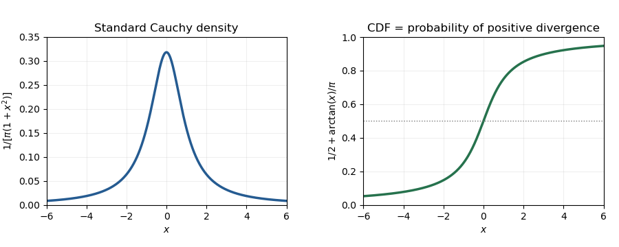
Standard Cauchy density and cumulative distribution, with the latter equal to the positive-divergence probability
. Details. Past exam of the mathematics course of the University of Cambridge 2015 iii Paper 30 5 b Solution by Codex 0 Created 2026-10-03 Updated 2026-10-14
Codex 0 Created 2026-10-03 Updated 2026-10-14The angle is a bounded local martingale, hence a uniformly integrable martingale. The martingale convergence theorem gives an almost sure and limit withIt must lie at an endpoint. Indeed, the Itô isometry and boundedness giveThus the bracket integral is finite almost surely. If the angle converged to an interior point, its squared cosine would eventually be bounded below by a positive constant, forcing this integral to be infinite. ConsequentlyThis proves endpoint convergence of a bounded angle diffusion.
Pinned article: Introduction to the OurBigBook Project
Welcome to the OurBigBook Project! Our goal is to create the perfect publishing platform for STEM subjects, and get university-level students to write the best free STEM tutorials ever.
Everyone is welcome to create an account and play with the site: ourbigbook.com/go/register. We belive that students themselves can write amazing tutorials, but teachers are welcome too. You can write about anything you want, it doesn't have to be STEM or even educational. Silly test content is very welcome and you won't be penalized in any way. Just keep it legal!
Intro to OurBigBook
. Source. We have two killer features:
- topics: topics group articles by different users with the same title, e.g. here is the topic for the "Fundamental Theorem of Calculus" ourbigbook.com/go/topic/fundamental-theorem-of-calculusArticles of different users are sorted by upvote within each article page. This feature is a bit like:
- a Wikipedia where each user can have their own version of each article
- a Q&A website like Stack Overflow, where multiple people can give their views on a given topic, and the best ones are sorted by upvote. Except you don't need to wait for someone to ask first, and any topic goes, no matter how narrow or broad
This feature makes it possible for readers to find better explanations of any topic created by other writers. And it allows writers to create an explanation in a place that readers might actually find it.
Figure 1. Screenshot of the "Derivative" topic page. View it live at: ourbigbook.com/go/topic/derivativeVideo 2. OurBigBook Web topics demo. Source. - local editing: you can store all your personal knowledge base content locally in a plaintext markup format that can be edited locally and published either:This way you can be sure that even if OurBigBook.com were to go down one day (which we have no plans to do as it is quite cheap to host!), your content will still be perfectly readable as a static site.
- to OurBigBook.com to get awesome multi-user features like topics and likes
- as HTML files to a static website, which you can host yourself for free on many external providers like GitHub Pages, and remain in full control

Figure 2. You can publish local OurBigBook lightweight markup files to either OurBigBook.com or as a static website.
Figure 3. Visual Studio Code extension installation.
Figure 5. . You can also edit articles on the Web editor without installing anything locally. Video 3. Edit locally and publish demo. Source. This shows editing OurBigBook Markup and publishing it using the Visual Studio Code extension. 
- Infinitely deep tables of contents:



All our software is open source and hosted at: github.com/ourbigbook/ourbigbook
Further documentation can be found at: docs.ourbigbook.com
Feel free to reach our to us for any help or suggestions: docs.ourbigbook.com/#contact