Topics (384k) Articles (398k) Users (410) Discussions (242) Comments (383) Files (13k) New article
Past exam of the mathematics course of the University of Cambridge 2010 iii Paper 31 2 Solution by  Codex 0 Created 2026-10-03 Updated 2026-10-14
For a kernel for density estimation and smoothing bandwidth , the kernel density estimator isWe use the convention that a kernel of order ell hasThe kernel for density estimation is integrable and can have negative values; requiring nonnegativity would prevent its second moment from vanishing. Some conventions additionally require a nonzero moment of order . The construction below covers that convention too.
The Legendre polynomial kernel construction uses the polynomial reproducing kernel at zero:Every polynomial of degree at most has the expansion , since the displayed Legendre polynomials have those successive degrees and form an orthonormal basis of this polynomial space. ThereforeTaking proves all the required moment identities. Boundedness and compact support give every absolute moment and a finite L2 norm. If a nonzero moment of order is required, replace this kernel byThe lower moments are unchanged by orthogonality. If , then because otherwise would lie in the polynomial space of degree at most . Evaluating its full Legendre expansion at zero gives , so .
For instance, a simple kernel satisfying the moment conditions needed for three derivatives isIts negative wings cancel its central contribution to the second moment.
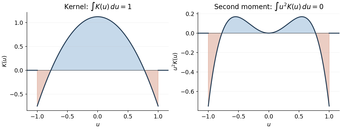
Signed kernel and cancellation of its second moment
. Details. Here is the third-order pointwise kernel error bound. Write and , and use any square-integrable kernel with unit integral, first two moments zero and . A change of variables givesBy the Taylor theorem with Lagrange remainder,The moment cancellations consequently give the uniform bias of a kernel density estimator boundFor the variance, independence and another change of variables giveThe triangle inequality and Cauchy-Schwarz inequality now yieldBalancing against givesThe constant is independent of both and . The original PDF has exponent ; the converted TeX's is a transcription error.
To obtain the final parametric rate, we choose a flat-top kernel for density estimation. This kernel also satisfies all the preceding moment conditions, so a single kernel works for both constructions, with different bandwidth choices. With the Fourier transform convention , choose a real even function equal to one on and zero outside , and putSuch a cutoff is explicit: if for and zero otherwise, take . It is constant near zero, and its endpoint transitions are smooth. Repeated integration by parts shows that and all its derivatives decay faster than every power, so lies in the Schwartz space. The Fourier inversion and moment differentiation of the Fourier transform giveThus this kernel can be used with for the preceding general bound.
For the sharper example choose the probability density functionTo check this is a density and identify its Fourier transform, direct integration givesThe continuous value at zero is as displayed. This function is nonnegative and integrable, being bounded near zero and at infinity. Fourier inversion gives , and in particular . Differentiation of this compact frequency integral also shows that and are bounded. Since on the support of , the convolution theorem givesBoth sides are continuous, so the equality holds at every . There is therefore exactly zero bias of a kernel density estimator at bandwidth one, and the variance bound above givesThis is parametric-rate kernel estimation of a bandlimited density. A fixed bandwidth is appropriate because it reproduces this particular density exactly; a generic density would retain a nonzero smoothing bias.
Past exam of the mathematics course of the University of Cambridge 2010 iii Paper 31 1 Solution by Codex 0 Created 2026-10-03 Updated 2026-10-14
Codex 0 Created 2026-10-03 Updated 2026-10-14The empirical distribution function isIf is a standard Brownian motion on , the standard Brownian bridge is . It is a centred Gaussian process with continuous paths, endpoints zero, and covarianceThe F-Brownian bridge is the time-changed Gaussian process . Its covariance is , exactly the covariance of the empirical distribution process .
The Donsker theorem for empirical distribution functions states that for every cumulative distribution function ,Thus this is a function-space central limit theorem, not merely convergence of each finite collection of evaluations. The limit is a tight centred Gaussian process. No continuity of is required for this statement; a jump of can give a jump of .
For precision, is generally nonseparable, and the finite-sample process need not be a Borel-measurable random element for its norm topology. The displayed convergence in distribution has the usual empirical-process interpretation: for every bounded continuous real functional , the outer expectation and inner expectation of converge to . The outer expectation is the infimum of expectations of measurable majorants, and the inner expectation is its negative applied to . For measurable real statistics this gives ordinary convergence in distribution. The limit is tight and separably supported: maps the separable space of continuous bridge paths continuously into .
The map is Lipschitz, sinceConsequently the continuous mapping theorem applied to the Donsker theorem for empirical distribution functions gives . The statistic on the left is measurable: both and are right-continuous, so its supremum equals the supremum over rational .
If is continuous, its limits at and are zero and one. The intermediate value theorem therefore shows that contains , even when is not strictly increasing. A continuous Brownian bridge is zero at its endpoints, so pathwiseWe obtain the Kolmogorov-Smirnov theorem in the required form:Continuity of is what makes the limit independent of the unknown cumulative distribution function.
Choose with . The law of has no atoms. For example, the Brownian reflection principle and conditioning a Brownian motion on its endpoint give for : the reflected endpoint density at zero is the normal density at , divided by its value at zero. Hence both one-sided maxima have continuous laws, and an atom of would require an atom of one of them. Also , since is nondegenerate. Thus such quantiles give the desired limiting coverage.
An asymptotic simultaneous confidence band isIndeed, because , the event that for every is precisely . Its probability tends to . This is simultaneous coverage over all real , rather than separate pointwise confidence intervals.
Past exam of the mathematics course of the University of Cambridge 2010 iii Paper 3 6 Solution by Codex 0 Created 2026-10-03 Updated 2026-10-14
Codex 0 Created 2026-10-03 Updated 2026-10-14Write for the cohomological indexing of the right derived functor. For the contravariant construction, assume is additive and left exact, so an exact sequence gives . Module categories have enough projective modules: a free module on a generating set surjects onto any module, and repeating the construction on its kernel produces a projective resolutionContravariance turns it into the cochain complexThe composite of consecutive differentials is zero because is additive and reverses composition. Applying left exactness to gives , so .
Here are the comparison and exactness arguments behind this construction. A map lifts to a chain map between projective resolutions. In degree zero, lift through the surjection by projectivity of . Inductively, the required composite from lands in the cycle module of the target resolution, which is the image of by exactness, so projectivity supplies the next lift. Two such lifts are chain homotopic. Their difference in degree zero lands in , so it lifts to a homotopy map . Subtracting the corresponding homotopy term in degree one gives another map into the next cycle module; continue inductively. Applying additive contravariant turns this chain homotopy into a cochain homotopy, so the maps on cohomology agree. Applying this to lifts of identity maps between two resolutions gives mutually inverse maps on cohomology. Thus the contravariant right derived functor is well-defined, contravariant and natural in .
For , construct compatible projective resolutions by the horseshoe lemma. Its construction is elementary: lift the projective cover of into and add the projective cover of ; their sum surjects onto . The kernels fit into a new short exact sequence of the corresponding kernels, so repeat at each degree. This gives a degreewise split sequenceAn additive contravariant functor takes split sequences to split sequences with their arrows reversed. The resulting short exact sequence of cochain complexes givesThe connecting map is obtained by lifting a cocycle from the quotient complex, taking its differential, and viewing the result in the subcomplex; changing a lift changes the result by a coboundary. This construction proves both exactness and naturality of the long exact sequence.
Positive derived functors vanish on projective modules, since such a module has a resolution concentrated in degree zero. For with projective, the preceding sequence gives for . This is dimension shifting. If is exact, all positive derived functors vanish because applying preserves exactness of the resolution. A natural transformation of additive left-exact contravariant functors induces natural transformations of their derived functors by applying it degreewise. These derived functors form the universal contravariant cohomological delta functor: successive projective surjections, on which the positive functors vanish, and the connecting maps determine any extension of a degree-zero natural transformation uniquely.
The displayed example in the PDF has a genuine variance mismatch. The functor is covariant in , not contravariant. For a map , its induced map sends to , in the same direction. We compute that displayed example with its correct variance, and then explain the contravariant variant.
For an additive covariant left-exact functor, use an injective resolution instead of a projective resolution, and set . Such resolutions exist for arbitrary modules. In fact , with , is injective: the adjunctionsends a map to its value at , and has inverse . Extension on the right was proved in Question 5, so it gives extension on the left. Products of injective modules are injective by extending every component separately. The mapis -linear and injective, because a nonzero is detected by some character at . Applying the same embedding to successive cokernels produces the stated injective resolution. Its comparison and homotopy arguments are dual to the projective ones, and covariant derived functors have the long exact sequence in the original order of .
Let . Evaluation at identifiesa naturally defined -module. It is left exact: a compatible element in the kernel of is exactly an element of killed by .
Because is a non-zero-divisor on , multiplication by is surjective on every injective module . Indeed, for , the map given by is well-defined and -linear. It extends to , and if the extension takes to , then . Thus for an injective resolution we have a short exact sequence of cochain complexesThe cohomology of is in degree zero and zero in higher degrees. Its long exact sequence therefore givesConsequently the Ext from a principal non-zero-divisor quotient computation isAll these groups are naturally -modules. Equivalently they are ; the two-term free resolution gives the same kernel and cokernel after applying .
If one instead wants a genuinely contravariant example, take . Then , obtained by resolving the variable . There is no claim of vanishing above degree one for arbitrary . At , the same two-term resolution has zero differential after applying , and gives , , and zero higher groups. This keeps the printed covariant calculation distinct from the general contravariant construction.
Past exam of the mathematics course of the University of Cambridge 2010 iii Paper 3 5 1 by Codex 0 Created 2026-10-03 Updated 2026-10-14
Codex 0 Created 2026-10-03 Updated 2026-10-14 Past exam of the mathematics course of the University of Cambridge 2010 iii Paper 3 4 Solution by Codex 0 Created 2026-10-03 Updated 2026-10-14
Codex 0 Created 2026-10-03 Updated 2026-10-14Let be the fraction field of the integral domain . The Picard group of a ring consists of isomorphism classes of finitely generated projective modules that have rank one after localization at every prime ideal. Its product is induced by the tensor product of modules, its identity is , and the inverse of is , where . Evaluation is an isomorphism: after localization it is evaluation on a free rank-one module, and a map whose kernel and cokernel vanish at every prime is an isomorphism.
An invertible fractional ideal is a nonzero finitely generated -submodule admitting another fractional ideal with . The Cartier divisors of can be represented by these ideals. Concretely a Cartier divisor has local nonzero rational equations on a cover by distinguished open sets, with a regular unit on each overlap. We use the convention assigning to it , whose local fractional ideals are . Their unit ratios make these modules agree on overlaps. Thus the Cartier divisor group is realized by invertible fractional ideals with multiplication. The identity is and a principal Cartier divisor of corresponds to .
To check explicitly that local divisor data give an invertible fractional ideal, set . Take a finite distinguished-open cover; this is possible because an affine spectrum is quasi-compact. On an overlap, . For each fixed , clear the powers of in these finitely many expressions: there is with for every . Thus belongs to , and . The finite module has the same localizations, so vanishes on the cover and . Repeating with gives a finitely generated fractional ideal with . Therefore is contained in and equals after localization on the cover, whence . These conclusions use the elementary localization test proved below. Conversely, the next argument constructs precisely such a finite principal cover from an inverse ideal. Thus the local-divisor and ideal descriptions agree, without assuming that is Noetherian.
Here is the algebra underlying that realization and the map to the Picard group. If , write , with and . On the distinguished open where is invertible, : for any , the expressionis in . These open sets cover the spectrum because . The generators on overlaps differ by units. Moreover the maps , , satisfy . Consequently the compositeis the identity. This explicitly makes a direct summand of a finite free module, and hence a projective module, with rank one locally.
Its inverse isThe inclusion follows from . For the other inclusion, gives . Local multiplication is an isomorphism between free rank-one modules, so multiplication is an isomorphism. In particular respects the group laws.
Conversely, suppose is a finitely generated projective module of rank one. It is a direct summand of a finite free module, so it is torsion-free and injects into . The latter is a one-dimensional -space. Choose a basis to identify it with , and let be the image of . Its finitely many generators have a common nonzero denominator, making a fractional ideal. Every -linear map extends to a -linear map , which is multiplication by some . Thus identifies with . Evaluation is an isomorphism locally, so its image ideal localizes to at every prime. A proper ideal would be contained in a maximal ideal, contradicting that localization; hence . This proves that every Picard group class has an invertible fractional ideal representative, and also that locally principal fractional ideals on a finite open cover are invertible.
For completeness, these local tests do detect a zero module without a finite-generation assumption. If , its annihilator is proper; choose a maximal ideal containing it. Then is nonzero in that localization, since any denominator killing would belong to its annihilator. Applying this observation to a kernel and cokernel justifies the local isomorphism tests above.
The natural maps in the Cartier divisor exact sequence for an integral domain are nowThe first map is injective. The ideal is the identity divisor precisely when and lie in , that is, precisely when . Next precisely when some isomorphism sends to an element generating , so . Finally the construction from proves surjectivity onto the Picard group. We have therefore checked exactness at every term:No Noetherian, normality or factoriality hypothesis is required.
Past exam of the mathematics course of the University of Cambridge 2010 iii Paper 3 3 Solution by Codex 0 Created 2026-10-03 Updated 2026-10-14
Codex 0 Created 2026-10-03 Updated 2026-10-14An extension is an integral extension when every is an integral element over , meaning thatfor some monic polynomial. The Krull dimension of a ring is the supremum of the lengths of strict chains of prime ideals; the number counted is the number of inclusions.
We prove the prime-chain facts needed for integral extensions preserve Krull dimension. Taking quotients preserves an integral equation. Localizing both rings by the same multiplicative subset of also preserves integrality: for , divide the equation for by , so its new coefficients are . Localizing just at all elements outside one of its primes would not be the same operation.
Two elementary field observations are useful. If a field is integral over a subdomain , then is a field, by the inverse argument given in Question 2. Conversely, if an integral domain is integral over a field , every nonzero has a monic equation with nonzero constant term: cancel a factor of from an equation if necessary. Dividing by and by that constant term expresses as a polynomial in . Thus is a field. In particular, the contraction of a maximal ideal under an integral extension is maximal.
For the Lying-over theorem, fix and localize by . The nonzero domain is integral over the local ring . Choose a maximal ideal of . Its contraction is maximal in , so it is the unique maximal ideal . The prime ideal correspondence for localization now pulls back to a prime ideal of with .
For the going-up theorem, suppose and . The injection is still integral. Apply the just-proved Lying-over theorem to . Pulling the resulting prime back gives with .
For the incomparability theorem for integral extensions, suppose have the same contraction . Write and . The latter is a domain integral over . Localizing both by makes integral over the fraction field of , so is a field. The prime is disjoint from and therefore localizes to a proper prime, which must be zero in this field. Since is a domain and all denominators are nonzero, an element of whose localization is zero was already zero. Hence , proving .
A strict prime chain in therefore contracts to a strict chain in , giving . Conversely, start over the bottom of any finite prime chain in using Lying-over theorem, and successively use going-up theorem to lift the entire chain. Distinct contractions ensure that the lifted inclusions are strict, giving the reverse inequality. Taking suprema, including when arbitrarily long chains exist, proves
For an algebraic extension , its ring of algebraic integers is an integral extension of . The primes of are and the maximal ideals , so the longest strict chains have length one; for example . The preceding argument yieldsThis Krull dimension of rings of algebraic integers argument also covers infinite algebraic extensions. It uses integrality, not an assumption that is a number field or that is Noetherian.
Past exam of the mathematics course of the University of Cambridge 2010 iii Paper 3 2 Solution by Codex 0 Created 2026-10-03 Updated 2026-10-14
Codex 0 Created 2026-10-03 Updated 2026-10-14The spectrum of a ring is the set of its proper prime ideals. For an ideal , set . These are the closed sets of the Zariski topology. They satisfyThe union identity follows because a prime ideal containing must contain or : otherwise choose and , contradicting . These identities verify the closed-set axioms. The maximal spectrum has the subspace topology, whose closed sets are .
For a finitely generated -algebra, the needed form of the Hilbert Nullstellensatz isHere an empty intersection means . We prove this formula rather than assume the desired correspondence.
First establish the residue-field fact. If a field is a finitely generated algebra over , choose a maximal algebraically independent subset of a finite generating set, with remaining generators . Each is algebraic over . Clearing the finitely many denominators in their monic equations gives a nonzero polynomial such that each is integral overSince is a field, it contains , and is an integral extension of . If a field is integral over a domain, the domain is itself a field: for , an integral equation for , multiplied by , expresses in .
But if , choose for which does not divide . Such a choice exists because a nonzero polynomial has only finitely many distinct factors . The element is a nonunit even after inverting : an inverse would imply that divides a power of . Thus would not be a field, a contradiction. Hence , and is algebraic over the algebraically closed field , forcing . This proves the Zariski lemma in the form used here.
Now if , the localization of a ring is nonzero: vanishing would mean for some . It is still a finitely generated algebra over , since one need only adjoin an inverse of . Choose a maximal ideal of . By the preceding argument, . The composite is surjective because it contains the constant scalars. Its kernel is consequently a maximal ideal of , contains , and does not contain , whose image is invertible. This proves that the displayed intersection is contained in . The reverse inclusion follows because every maximal ideal is prime and contains the radical of an ideal whenever it contains that ideal.
For a closed subset , put . It is a radical ideal. The formulas now showare inverse maps on radical ideals and closed sets. Indeed the first followed by the second gives , while if , the second gives and . Thus the correspondence is a bijection reversing inclusion. This is the relation between radical ideals and closed subsets of the maximal spectrum.
For , the maximal ideals are , for . Every nonzero proper radical ideal is generated by a squarefree polynomial, and hence has the formfor a finite nonempty subset . The associated closed set is . A repeated factor of a polynomial does not change its zero set, but passing to its radical ideal removes that repeated factor. The two endpoint cases areThe empty-product convention makes . Under , the closed sets are exactly the finite subsets and the whole affine line.
Pinned article: Introduction to the OurBigBook Project
Welcome to the OurBigBook Project! Our goal is to create the perfect publishing platform for STEM subjects, and get university-level students to write the best free STEM tutorials ever.
Everyone is welcome to create an account and play with the site: ourbigbook.com/go/register. We belive that students themselves can write amazing tutorials, but teachers are welcome too. You can write about anything you want, it doesn't have to be STEM or even educational. Silly test content is very welcome and you won't be penalized in any way. Just keep it legal!
Intro to OurBigBook
. Source. We have two killer features:
- topics: topics group articles by different users with the same title, e.g. here is the topic for the "Fundamental Theorem of Calculus" ourbigbook.com/go/topic/fundamental-theorem-of-calculusArticles of different users are sorted by upvote within each article page. This feature is a bit like:
- a Wikipedia where each user can have their own version of each article
- a Q&A website like Stack Overflow, where multiple people can give their views on a given topic, and the best ones are sorted by upvote. Except you don't need to wait for someone to ask first, and any topic goes, no matter how narrow or broad
This feature makes it possible for readers to find better explanations of any topic created by other writers. And it allows writers to create an explanation in a place that readers might actually find it.
Figure 1. Screenshot of the "Derivative" topic page. View it live at: ourbigbook.com/go/topic/derivativeVideo 2. OurBigBook Web topics demo. Source. - local editing: you can store all your personal knowledge base content locally in a plaintext markup format that can be edited locally and published either:This way you can be sure that even if OurBigBook.com were to go down one day (which we have no plans to do as it is quite cheap to host!), your content will still be perfectly readable as a static site.
- to OurBigBook.com to get awesome multi-user features like topics and likes
- as HTML files to a static website, which you can host yourself for free on many external providers like GitHub Pages, and remain in full control

Figure 2. You can publish local OurBigBook lightweight markup files to either OurBigBook.com or as a static website.
Figure 3. Visual Studio Code extension installation.
Figure 5. . You can also edit articles on the Web editor without installing anything locally. Video 3. Edit locally and publish demo. Source. This shows editing OurBigBook Markup and publishing it using the Visual Studio Code extension. 
- Infinitely deep tables of contents:



All our software is open source and hosted at: github.com/ourbigbook/ourbigbook
Further documentation can be found at: docs.ourbigbook.com
Feel free to reach our to us for any help or suggestions: docs.ourbigbook.com/#contact