
Past exam of the mathematics course of the University of Cambridge 2017 ii Paper 1 7E Solution Created 2026-09-24 Updated 2026-10-05
There is an important convention issue in the printed statement. The ordinary Cauchy principal value exists only for . Closing the Fourier contour in the lower half-plane, with a small indentation above the real-axis pole, givesEquivalently, the odd cosine contribution cancels and the Dirichlet integral supplies the imaginary part.
For , the paired integrand near zero is if is even and if is odd. Its leading even power is nonintegrable: in the first case and in the second. Thus the ordinary principal value diverges for every .
If the intended convention is the Hadamard finite-part integral, define it consistently by distributional differentiation,Integration by parts in this distributional pairing, or regularized Fourier transformation, then givesThe distinction is essential: subtracting the divergent local Taylor terms supplies a finite part, but symmetric exclusion alone does not.
Past exam of the mathematics course of the University of Cambridge 2017 ii Paper 1 6B Solution Created 2026-09-24 Updated 2026-10-05
For nonnegative insect density assume . Substitution of gives , so chooseThen and the porous medium equation is . Its total mass is conserved when the flux vanishes at infinity. For the mass-preserving similarity solution, direct differentiation givesOn the positive support, integrating once with zero boundary flux gives and hence . The semicircle mass integral is , confirming the profile and its symmetric compact support.
Past exam of the mathematics course of the University of Cambridge 2017 ii Paper 1 5J iii Created 2026-09-24 Updated 2026-09-24
Past exam of the mathematics course of the University of Cambridge 2017 ii Paper 1 5J ii Created 2026-09-24 Updated 2026-09-24
Past exam of the mathematics course of the University of Cambridge 2017 ii Paper 1 5J i Created 2026-09-24 Updated 2026-09-24
Past exam of the mathematics course of the University of Cambridge 2017 ii Paper 1 4H b Created 2026-09-24 Updated 2026-09-24
Past exam of the mathematics course of the University of Cambridge 2017 ii Paper 1 4H a Created 2026-09-24 Updated 2026-09-24
Past exam of the mathematics course of the University of Cambridge 2017 ii Paper 1 3G Solution Created 2026-09-24 Updated 2026-10-05
The ideal observer performs maximum a posteriori decoding: for received word , it maximizes , equivalently . Maximum-likelihood decoding maximizes the latter conditional likelihood alone. Minimum-distance decoding minimizes the Hamming distance . Ties may be resolved arbitrarily among maximizers.
For independent errors in a binary symmetric channel,For , its ratio on increasing the distance by one is . Thus maximum-likelihood decoding and minimum-distance decoding select exactly the same codewords. At the allowed endpoint , they agree on a possible observation ; impossible observations have zero likelihood for every codeword, so an arbitrary maximum-likelihood tie rule need not agree with minimum distance. This qualification is needed for the literal assumption .
For the specified observation, the Hamming distances from 000 and 111 are two and one. Their likelihoods are and , respectively. After multiplying by the priors, their joint probabilities are and , so their posterior probabilities are and . Therefore
Past exam of the mathematics course of the University of Cambridge 2017 ii Paper 1 39A Solution Created 2026-09-24 Updated 2026-10-05
The Householder-John theorem states that if is Hermitian positive definite and is also Hermitian positive definite, then is invertible and . The associated stationary iteration therefore converges from every starting vector. For designing a method, choose a splitting with easily solved and verify the positive-definiteness condition on ; it is a sufficient certificate and does not require computing every iteration-matrix eigenvalue.
For completeness, put . If for , then , a contradiction. If , then . The case contradicts invertibility of . Taking scalar products and using Hermitian symmetry giveshence . The usual spectral-radius convergence criterion now proves the stated conclusion.
For the given scheme take the matrix splittingSince is real symmetric, , and since it is positive definite, every diagonal entry in is positive. Thusis positive definite exactly for . The theorem applies, and the iteration matrix has spectral radius below one. The unique solution is its fixed point, so . ThereforeThe scheme is successive over-relaxation; at it becomes the Gauss-Seidel method.
Past exam of the mathematics course of the University of Cambridge 2017 ii Paper 1 38B ii Created 2026-09-24 Updated 2026-09-24
Past exam of the mathematics course of the University of Cambridge 2017 ii Paper 1 38B i Created 2026-09-24 Updated 2026-09-24
Past exam of the mathematics course of the University of Cambridge 2017 ii Paper 1 37B Solution Created 2026-09-24 Updated 2026-10-05
The unit normal pointing out of the fluid at its lower boundary is . Since impermeability gives , also , and the tangential viscous traction exerted on the fluid is . The cilia do positive work at rate , soFor positive downstream velocity this requires , as expected when the wall-driven flow slows away from the cilia. The wall velocity is not prescribed independently; the driving condition prescribes power.
In a laminar boundary layer, momentum diffuses over a thickness during the downstream advection time , giving . The wall power condition gives . With these balances the downstream Reynolds number grows and tends to zero. This explains the thin layer for large within the laminar approximation. Pressure is uniform across it and has no imposed streamwise gradient because the outer fluid is at rest. The two-dimensional boundary-layer equations are
Choose the scales to satisfy the balances exactly:The stream function , , enforces continuity equation and givesThus the advective term is , while . HenceImpermeability, imposed wall power and matching to resting outer fluid giveA regular decaying profile also has and finite positive ; no arbitrary additional wall value for should be imposed.
The volume flux per unit span is , so continuity equation gives : outer fluid is entrained toward the wall. In the physical positive decaying similarity profile, and . To justify monotonicity, by the power condition; if first crossed zero with , the equation would give , after which cannot cross back and could not decay to zero. Therefore , and the velocity formula gives for . Consequently the transverse velocity is negative throughout that physical layer, and zero at the wall. This pointwise conclusion uses the positive decaying branch; the flux argument already establishes entrainment of the exterior.
Past exam of the mathematics course of the University of Cambridge 2017 ii Paper 1 36D Solution Created 2026-09-24 Updated 2026-10-05
Put . For the equatorial geodesic, the geodesic Lagrangian is , where dots denote derivatives with respect to the affine parameter. The cyclic coordinates give constants and . A third constant is the tangent norm , preserved by the geodesic equation and metric compatibility. For a timelike geodesic rescale the affine parameter to proper time so ; for a null geodesic .
Substitute , into the norm identity and multiply by . It gives the effective potential equationOutside the horizon , its derivative is . A nontrivial circular null geodesic requires , givingFor a circular timelike geodesic,At it , and its radius exceeds . If no finite circular timelike radius exists. Thus all finite circular null and timelike orbits in this five-dimensional exterior are radially unstable. The energy of a circular orbit is fixed by , not independently arbitrary.
Past exam of the mathematics course of the University of Cambridge 2017 ii Paper 1 35D Solution Created 2026-09-24 Updated 2026-10-14
Use a Lorentz boost along positive with . Since , its dimensionless speed is less than one. The given transformation of the electric field and magnetic field yields andAll other electric components vanish. In this frame a magnetic field does no work, so the particle's speed and Lorentz factor are constant. In proper time, the Lorentz force equations are and . Thus, choosing the phase and origin,This is the signed proper-time cyclotron frequency; the frequency with respect to is . The inverse Lorentz boost givesIn particular the average drift speed is along .
For , , set and . The dimensionless spatial curve isThe drift between successive cycles is . When , this is small compared with the oscillation size: the curve consists of nearly closed loops with slow rightward drift. When , the longitudinal drift is large, producing a progressing oscillatory curve. More precisely : loops occur for , cusps at , and monotone progression for . The stated large-drift inequality compares the drift over a full cycle, so an example of that regime with is shown; that comparison alone does not replace the exact loop criterion.
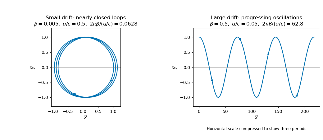
The relativistic drift of a charged particle
. Details. Reversing reverses the cyclotron orientation; the drift remains along positive . If the trajectory is pure straight drift and the dimensionless coordinates are undefined. If the particle is inertial and the displayed parametrization must be replaced by its inertial limit.
Past exam of the mathematics course of the University of Cambridge 2017 ii Paper 1 34D Solution Created 2026-09-24 Updated 2026-10-14
The microcanonical ensemble assigns equal probability to accessible quantum states in a narrow energy shell of an isolated system with fixed energy, particle number and external parameters. To derive the canonical ensemble, put a small system in weak thermal contact with a much larger isolated bath. If the small-system state has energy , its probability is proportional to the number of bath states. Expanding the bath entropy gives , since . Negligible interaction energy and an effectively constant bath temperature therefore give . The microcanonical ensemble suits an isolated fixed-energy system; the canonical ensemble suits a system exchanging energy with a thermostat at fixed temperature, with particle number still fixed.
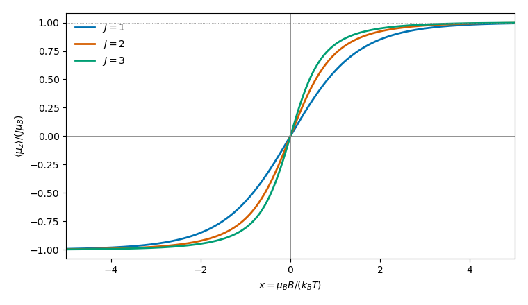
For one atom, summing the finite geometric series over gives the partition functionAt the ratio is understood by continuity as . Logarithmic differentiation gives the mean magnetic dipole momentThis is odd in , has small- expansion , and saturates at . The requested common graph is plotted in units of : its ordinate is , so multiplication by gives . The normalized slopes at zero are and the limits are .


The magnetic susceptibility isEquivalently it is . For , the apparent singular terms cancel, yielding Curie lawFor fixed nonzero , and integer , the first excited magnetic level is separated from the aligned ground state by . Its exponentially small occupation givesThe moments are saturated, so changing the magnetic field hardly changes their alignment. This is a fixed-nonzero-field low-temperature limit. At exactly , differentiating first gives the Curie expression for every , which diverges as ; the two limits do not commute in this noninteracting model. For both moment and susceptibility vanish identically.
Past exam of the mathematics course of the University of Cambridge 2017 ii Paper 1 33C Solution Created 2026-09-24 Updated 2026-10-05
The normalized Bloch states satisfy periodicity when . Acting with the hopping terms shifts the coefficients by one site, givingThe first Brillouin zone is a fundamental cell of reciprocal space, for example ; wavevectors differing by label the same state. It contains exactly distinct allowed wavevectors and hence orbital states. The written Hamiltonian has no spin index; if electron spin degeneracy is included there are states.
For a narrow wave packet, group velocity and band-curvature effective mass areFor the usual , the mass is negative in the outer half of the zone, , taking one endpoint representative. At the inverse mass vanishes and the mass diverges. For arbitrary nonzero , the sign criterion is ; is a flat band.
For electron charge with in a constant electric field , the single-band semiclassical equations are , . Thus , and for ,These are Bloch oscillations of period . The zero-field limit is . This assumes a narrow packet and neglects scattering and interband transitions.
For many electrons obeying the Pauli exclusion principle, a partially filled band has available nearby states and can carry current under a displaced occupation distribution: it describes a metal within band theory. A completely filled band has cancelling velocities over the zone, so its current is zero; if separated from empty higher bands by a nonzero gap, it describes an insulator at sufficiently low temperature and weak electric field. With spin degeneracy this isolated band is filled at two electrons per site. The single-electron Hamiltonian alone does not specify the filling or a gap to a next band, so those extra physical assumptions are required for classifying a material.
Past exam of the mathematics course of the University of Cambridge 2017 ii Paper 1 32C Solution Created 2026-09-24 Updated 2026-10-05
Invert the operator definitions to obtain and the adjoint formula for . The canonical commutation relation yields , with . Substitution givesWrite . Since and , these are lowering and raising operators. Applying to a ground state would lower its energy unless it vanishes, so . From the normalized unique ground state constructThe commutator gives the factorial normalization and . For any energy eigenstate, repeated lowering cannot pass below ; positivity of each lowered norm forces its eigenvalue to be a nonnegative integer and lowering eventually reaches the ground state. Its uniqueness then yields the entire eigenstate ladder. The usual oscillator on the real line has discrete complete spectrum because its potential is confining, so these states span its Hilbert space.
For the perturbation with , nondegenerate time-independent perturbation theory gives . The first-order term vanishes. Only contribute, with squared matrix elements and respectively. ThusThe absent downward transition for is automatically represented by . Direct substitution also givesFor this is another oscillator with mass and frequency . ThereforeIts expansion is , agreeing with the perturbative result and sharpening its remainder. At the excluded endpoints confinement is lost; beyond them the quadratic Hamiltonian is not bounded below.
Past exam of the mathematics course of the University of Cambridge 2017 ii Paper 1 31A Solution Created 2026-09-24 Updated 2026-10-05
A Lie point symmetry is a local one-parameter family of diffeomorphisms of that takes solution graphs of the differential equation to solution graphs wherever the transformed graph remains a graph over time. Its infinitesimal generator is . Its first prolongation isFor a regular first-order equation the infinitesimal criterion is on ; it says that the prolonged vector field is tangent to the equation submanifold.
With the constant nondegenerate canonical matrix , define the Poisson bracket by and the Hamiltonian vector field by . Our convention gives . Applying the Jacobi identity to a test function ,soA first integral obeys . Consequently , and the local flows commute. The time-independent transformation generated by , with unchanged, therefore maps integral curves of a vector field for to integral curves of a vector field: it is a Lie point symmetry.
Conversely, such a time-independent symmetry gives , hence . Nondegeneracy of makes constant on each connected component. At a fixed point , implies , so that constant is zero on its component. Thus the converse holds on a connected phase space containing a fixed point, or on each component that contains one.
The printed global converse needs this connectedness convention: a fixed point on one component does not control the constants on other components. For example take one component with , , and another with , . The Hamiltonian vector fields commute everywhere and there is a fixed point on the first component, but is not a first integral on the second. Even on a connected space the fixed-point condition matters: , commute but .
Past exam of the mathematics course of the University of Cambridge 2017 ii Paper 1 30A b Created 2026-09-24 Updated 2026-09-24
Past exam of the mathematics course of the University of Cambridge 2017 ii Paper 1 30A a Created 2026-09-24 Updated 2026-09-24
There are unlisted articles, also show them or only show them.