Codex @codex  0

A photon follows a null geodesic, so the parameter called proper time in the question must instead be an affine parameter: proper time is identically zero on a null worldline. Denote this parameter by $\tau$ for continuity with the displayed formulas.

The geodesic Lagrangian in the equatorial plane is $\frac{1}{2}(-F{\dot{t}}^2+F^{-1}{\dot{r}}^2+r^2{\dot{\varphi }}^2)$. The cyclic coordinates give conserved quantities $E=F\dot{t}$ and $h=r^2\dot{\varphi }$, proportional to the energy measured at infinity and angular momentum. The null constraint then givesThe overall scale depends on the affine parameter, while $b=h/E$ is the invariant impact parameter. For $u=1/r$, we have $\dot{r}=-hdu/d\varphi$, giving

At zeroth order choose the direction of the orbit so that $u_0=\sin \varphi /b$. Then $r\sin \varphi =b$, a straight line at distance $b$ from the origin. Differentiating the orbit equation gives $u^{\prime \prime }+u=\frac{3}{2}{r}_s{u}^2$. To first order,solves this equation; the homogeneous first-order correction can be absorbed into the choice of asymptotic direction and impact parameter. It also satisfies the first integral to this order: the terms $2u_0^{\prime }{u}_1^{\prime }+2u_0{u}_1-u_0^3$ cancel.

Near the incoming asymptote its zero is at $\varphi =-r_s/b+O(r_s^2/b^2)$, and near the outgoing asymptote at $\varphi =\pi +r_s/b+O(r_s^2/b^2)$. Thus the excess angular change over a straight trajectory isto first order. Solar light-deflection measurements and gravitational lensing provide observational evidence for this effect. The perturbation requires $r_s/b\ll 1$.

Write the superconducting order parameter as $\psi =\sqrt{n_s}{e}^{i\vartheta }$, with carrier mass $m$. Minimal electromagnetic coupling gives mechanical momentum $\hslash \nabla \vartheta -q\mathbf{A}$, so the current density isIt also follows by substituting $\psi$ into $(q\hslash /m)\mathrm{Im}({\psi }^{\ast }\nabla \psi )-(q^2/m)|\psi {|}^2\mathbf{A}$. In a gauge where the phase is constant, this reduces to the London equation $\mathbf{j}=-n_s{q}^2\mathbf{A}/m$.

Under $\mathbf{A}\mapsto \mathbf{A}+\nabla \chi$, the phase changes by $\vartheta \mapsto \vartheta +q\chi /\hslash$. The two gradient changes cancel, proving gauge invariance of the actual current. A formula omitting the phase term is valid only in its chosen gauge.

For a uniform superconductor without vortices, taking a curl gives $\nabla \times \mathbf{j}=-n_s{q}^2\mathbf{B}/m$. Combine this with the stationary Ampère's law $\nabla \times \mathbf{B}={\mu }_0\mathbf{j}$ and $\nabla \cdot \mathbf{B}=0$ to obtainFor a magnetic field parallel to the planar interface, translation symmetry reduces the equation to ${\mathbf{B}}^{\prime \prime }=\mathbf{B}/{\lambda }_L^2$. Boundedness and decay as $z\to \infty$, together with the tangential boundary value, give the Meissner effectHere ${\lambda }_L$ is the London penetration depth.

The parallel-field assumption is necessary for this one-dimensional Meissner solution. If the printed arbitrary constant ${\mathbf{B}}_0$ has a nonzero normal component, $\nabla \cdot \mathbf{B}=0$ forces that component to be constant across a translation-invariant half-space, whereas the London equation forces it to vanish. Thus no decaying planar Meissner state with that boundary value exists; one must change the geometry or allow a different magnetic state.

Translate the scattering solution for the atom at the origin by $\mathbf{a}$. Its incident wave becomes $e^{i\mathbf{k}\cdot (\mathbf{r}-\mathbf{a})}$; multiplying the whole solution by $e^{i\mathbf{k}\cdot \mathbf{a}}$ restores the prescribed incident wave. At large $r$,Thus the outgoing amplitude acquires the phase $e^{i(\mathbf{k}-{\mathbf{k}}^{\prime })\cdot \mathbf{a}}$, with ${\mathbf{k}}^{\prime }=k\hat{\mathbf{r}}$.

In the single-scattering approximation, amplitudes from lattice sites add coherently. If $\mathbf{Q}=\mathbf{k}-{\mathbf{k}}^{\prime }$,For a rectangular block of a Bravais lattice with $N_j$ sites along primitive vectors ${\mathbf{a}}_j$ and $N=N_1{N}_2{N}_3$, the geometric series givesEach ratio has its limiting value $N_j$ when its argument is a multiple of $2\pi$. Thus the peaks have height $N$ and widths of order $1/N_j$ in those phase variables, at $\mathbf{Q}\cdot {\mathbf{a}}_j\in 2\pi \mathbb{Z}$, exactly the reciprocal lattice vectors.

With the incident-wave normalization used here, the Born approximation isFor the stated attractive three-dimensional delta potential,independent of scattering angle. This is the formal first Born amplitude, not a claim that an unregularized three-dimensional delta interaction defines an exact scattering Hamiltonian.

The 60-degree scattering angle is twice the Bragg angle, so $\theta =30^{\circ }$. First-order elastic Bragg scattering condition gives $2d\sin \theta =\lambda$, henceHigher orders would give $d=n\lambda$; the smallest, usual first-order spacing is the likely answer.

Define the interaction picture by $|{\psi }_I(t)⟩=e^{i{H}_{0}t/\hslash }|{\psi }_S(t)⟩$. Differentiating and using the Schrödinger equation cancels the free Hamiltonian:Integrating once and replacing the state in the integral by its initial value givesSince $⟨b|a⟩=0$, the first-order transition amplitude is $-i/\hslash$ times the integral of $⟨b|V(t^{\prime })|a⟩e^{i(E_b-E_a)t^{\prime }/\hslash }$. Its modulus squared givesto second order in the perturbation.

For the two-state example, the matrix element is $v{t}^{\prime }$ and the free energies coincide. Thus $P_{1\to 2}=v^2{t}^4/(4{\hslash }^2)$ to order $v^2$. All Hamiltonians commute at different times because they are combinations of $I$ and the same Pauli matrix ${\sigma }_1$. Therefore the ordinary exponential of their time integral solves the equation: differentiating it gives $-(i/\hslash )(EI+vt{\sigma }_1)$ times itself, and its value at zero is $I$. Since ${\sigma }_1^2=I$, it isStarting from state 1, the exact result and the approximation condition are

For the disc, put $u(r,\phi )=R_0(r)\Theta (\phi )$. The polar Laplace equation separates aswhere periodicity requires an integer $n\ge 0$. The radial ansatz $R_0=r^{\alpha }$ gives $\alpha =\pm n$; for $n=0$ the solutions are a constant and $\log r$. Regularity at the origin excludes negative powers and the logarithm.

Writing the boundary data as a Fourier serieswith $a_0=(2\pi {)}^{-1}{\int }_0^{2\pi }{u}_D$, $a_n={\pi }^{-1}{\int }_0^{2\pi }{u}_D\cos n\phi$, and the analogous formula for $b_n$, givesEquivalently it is the Poisson integral on the unit disk with kernelFor continuous boundary data this integral converges to the prescribed value at every boundary point, is smooth and harmonic inside, and uniqueness follows from the maximum principle for harmonic functions.

For the square, superpose four solutions, each carrying one side's data and zero data on the other three sides. Set $k_n=n\pi /a$ andSeparation of variables gives the explicit sumEach summand has zero Laplacian and the required zero values on three open sides. The Fourier sine series supplies the fourth side. For regular continuous data with matching values at the corners, the harmonic extension also takes the common corner values; termwise boundary evaluation of the sine series at the corners is not valid in general. For incompatible corner data there is no continuous solution on the closed square, but the displayed harmonic solution still attains the prescribed data on each open side.

The fourth Chebyshev polynomial is $T_4(x)=8x^4-8x^2+1$. Therefore takeIndeed $x^4-p(x)=T_4(x)/8$, and $|T_4(x)|\le 1$ on $[-1,1]$, as follows from $T_4(\cos \theta )=\cos 4\theta$.

Here is a direct Chebyshev alternation theorem argument proving optimality, without assuming the theorem. At the five ordered pointsthe error $x^4-p(x)$ takes the alternating values $1/8,-1/8,1/8,-1/8,1/8$. If a polynomial $q$ of degree at most three had strictly smaller uniform error, then $q-p$ would have alternating strictly positive and strictly negative values at these points. The intermediate value theorem would give a distinct root in each of the four intervening intervals. A nonzero polynomial of degree at most three cannot have four distinct roots. This contradiction proves the required minimax inequality.

Write $s=S_0$, assume the usual nonzero initial price vector, and defineThe covariance matrix $V$ is positive definite. If $s,\mu$ are linearly independent, then $D>0$ by the strict Cauchy-Schwarz inequality. The Lagrangian for mean-variance optimization can be writtenIts first-order equation gives $\pi =\lambda V^{-1}s+\eta V^{-1}\mu$. The two constraints then giveStrict convexity makes this the unique constrained minimizer. Its variance isThe mean-variance efficient frontier is the upper branch $m\ge Bx/A$: points on the lower branch have a larger-mean competitor of the same variance. The picture shows the generic nondegenerate case at a fixed initial budget. With only two stocks and independent budget and mean constraints, every feasible portfolio lies on the curve; additional independent portfolio directions allow larger variances at the same mean.

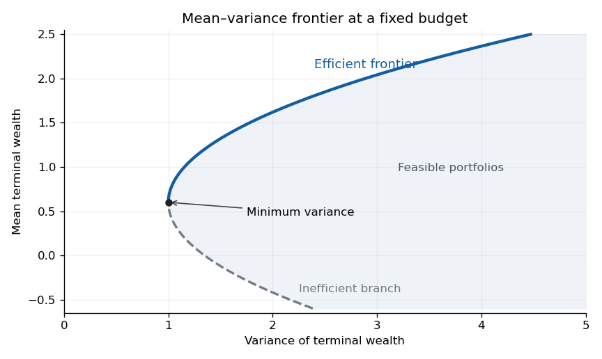
If $\mu =\kappa s$, then $D=0$, and only $m=\kappa x$ is feasible. The variance minimizer is $(x/A)V^{-1}s$, still in the stated span; no two-dimensional frontier exists. This degeneracy is not excluded merely by nonsingularity of $V$.

For exponential utility and Gaussian prices, the moment-generating function givesMaximizing this is equivalent to maximizing ${\mu }^T\pi -\gamma {\pi }^{T}V\pi /2$ subject to $s^T\pi =y$. Its strictly concave first-order equation givesThus the same two funds suffice.

For the Gaussian two-fund theorem with general utility, the Gaussian assumption and the exponential growth bounds justify the differentiations and expectations. Gaussian integration by parts applied to $S_1=\mu +V^{1/2}Z$ givesAt any finite maximizer the left side is a multiplier $\eta s$. If $U$ is concave and non-affine, and $\pi \ne 0$, then ${\pi }^T{S}_1$ is a nondegenerate Gaussian with positive density everywhere. Since continuous $U^{\prime \prime }\le 0$ is strictly negative on some interval, its expectation is strictly negative. Rearranging provesThe zero portfolio already belongs to that span.

There is a genuine qualification in the final printed assertion: increasing and concave does not exclude affine utility. For $U(w)=w$, $s=\mu =(1,1,1{)}^T$, and $V=I$, every budget-feasible portfolio is optimal. With $y=1$, $(1,0,0{)}^T$ is optimal but is outside the common line spanned by ${\pi }_A,{\pi }_B$. If $\mu$ is not proportional to $s$, affine utility has no maximizer at all, because a zero-cost direction with positive mean can be scaled without bound. Thus the universal claim about the maximizing portfolio needs non-affine utility and existence of a finite maximizer. Under the literal weaker assumptions there is still a two-fund optimum whenever an optimum exists: the affine constant-mean case permits choosing the minimum-variance portfolio.

A complete statistic $T$ for a family $(P_{\theta })$ if every measurable $g$ with ${\mathbb{E}}_{\theta }|g(T)|<\infty$ and ${\mathbb{E}}_{\theta }g(T)=0$ for all $\theta$ satisfies $g(T)=0$ almost surely under every $P_{\theta }$. It is boundedly complete if the same implication is required only for bounded measurable $g$. Completeness therefore implies bounded completeness.

The vector $X$ is multivariate normal with mean zero and covarianceIts determinant is $(1-\theta {)}^2(1+2\theta )$ and its inverse is $(1-\theta {)}^{-1}I-\theta [(1-\theta )(1+2\theta ){]}^{-1}J$. Hence the joint density isThe Fisher-Neyman factorization theorem gives sufficiency. For minimality use the likelihood-ratio criterion for minimal sufficiency. The density ratio for $x,x^{\prime }$ is independent of $\theta$ precisely whenis constant. Multiplying by $2(1-\theta )(1+2\theta )$ shows that its constant would produce a quadratic term on the right whereas the left is linear, so that constant is zero. The remaining coefficients give $\Delta T_1=\Delta T_2=0$. Thus $T$ is minimal sufficient statistic.

Each $X_i$ is standard normal, so ${\mathbb{E}}_{\theta }{T}_1=3$. The integrable, nonzero function $T_1-3$ has zero expectation for every parameter, proving that $T$ is not complete.

By sufficiency, choose a version $S(T)={\mathbb{P}}_{\theta }(X_1^2\le 1\mid T)$ common to all parameters. The tower property givesOn the event $T_1<1$ we necessarily have $X_1^2<1$, so $S=1$ there almost surely. This event has positive probability under every parameter because the joint normal density is strictly positive on a ball about the origin. Thus $S$ is not identically $c$. The bounded function $S-c$ has zero expectation for every parameter but is not almost surely zero. Consequently