
Past exam of the mathematics course of the University of Cambridge 2008 ii Paper 4 9B a Created 2026-09-24 Updated 2026-09-24
Past exam of the mathematics course of the University of Cambridge 2008 ii Paper 4 8C Solution Created 2026-09-24 Updated 2026-10-14
Consider , extending it at zero by . It is holomorphic in the upper half-plane and on its boundary, and on large upper semicircles because . For real , indent the upper-half-plane contour above the pole of . The clockwise indentation contributes , while the large semicircle contributes zero in the limit. The Cauchy integral theorem givesWith the stated Hilbert transform convention this is . ButTaking real parts yields the Hilbert transform of the sinc function:At the right side has limit zero; the same value follows by oddness of the principal-value integrand. The apparent singularity of at zero is removable, so the contour calculation is valid there too.
Past exam of the mathematics course of the University of Cambridge 2008 ii Paper 4 7A Solution Created 2026-09-24 Updated 2026-10-14
In Glendinning chaos, a continuous interval map is chaotic when some positive iterate has a horseshoe for an interval map. In the interval version, one may take an open interval containing two disjoint open intervals with .
Let a three-cycle be ordered . There are only two possible cyclic orderings; reflection of the coordinate interchanges them, so assume , , . ThenAlso and , so the intermediate value theorem gives with , whence . Both and therefore map across under .
To obtain exact open-interval images, use the following elementary first-passage observation. A continuous function on with endpoint values has a subinterval on which its endpoint values are and all interior values lie strictly between them: take the first hit of the second level, then the last hit of the first level before it. The intermediate value theorem makes its interior image exactly . Apply this to the two intervals, reversing endpoint order on the first. Their selected interiors and are disjoint and lie in , withThis proves the three-cycle forces a two-iterate interval horseshoe result and establishes the required horseshoe for .
Past exam of the mathematics course of the University of Cambridge 2008 ii Paper 4 6B Solution Created 2026-09-24 Updated 2026-10-14
Balancing the viscous and bending terms gives , so the elastohydrodynamic penetration length isInserting into the linear equation yields , with , and decay at infinity. Write , . Of the four roots of , precisely two have negative real part:The two decaying solutions are and , and the general decaying response is their linear combination. Both coefficients are nonzero: if one vanished, would force the other to vanish, contradicting .
Their real parts in the time-dependent response are proportional toConstant phases move respectively with velocities and , so these are damped travelling waves moving left and right. Since , the right-going wave has the longer attenuation length and dominates at large . Thus the less strongly damped, outward-moving wave dominates the far-field response. This is the oscillatory bending of a moment-free semi-infinite filament; the two boundary conditions determine its amplitudes without needing them explicitly here.
Past exam of the mathematics course of the University of Cambridge 2008 ii Paper 4 5J Solution Created 2026-09-24 Updated 2026-10-14
These are nested Poisson regression models with independent counts and the default log link function. If is biomass and is the three-level pH group, model 1 specifies : one common intercept and slope. Model 2 specifies : three group-specific intercepts and a common slope. Model 3 specifies : three intercepts and three slopes, because the multiplication syntax includes both main effects and their interaction. The parameter counts are therefore .
The analysis of deviance compares model 1 against model 2 by testing equality of the three intercepts, conditional on a common biomass slope. The likelihood-ratio test statistic is with two additional parameters, giving the reported tiny p-value. The next test compares model 2 against model 3 by testing equality of their three slopes. Its statistic is , again with two degrees of freedom and reported . Both restrictions are rejected. Thus model 3 is the supported choice: both baseline richness and its biomass dependence vary with pH. Under the Poisson assumptions, residual deviance on residual degrees of freedom is also consistent with a satisfactory fit, although these nested tests themselves establish improvement rather than every possible aspect of model adequacy.
The prediction from model 2 is on its linear-predictor scale. Exponentiating gives its fitted means. The final expression is twice the saturated log likelihood minus the model-2 log likelihood, i.e. the Poisson deviance of model 2. ConsequentlyIn the saturated model each mean equals the corresponding observed count, with the usual continuous convention for a zero count.
Past exam of the mathematics course of the University of Cambridge 2008 ii Paper 4 4G Solution Created 2026-09-24 Updated 2026-10-14
A binary cyclic code is a linear subspace of invariant under cyclic coordinate shift. Associate a word to in . Cyclic shift is multiplication by , so linearity and shift invariance make the code an ideal of this quotient.
Its inverse image in is an ideal containing . Since a polynomial ring over a field is a principal ideal domain, that inverse image is for a unique monic polynomial . Containment gives for some polynomial . Thus the generator polynomial of a cyclic code satisfiesFor a nonzero code is also its monic word polynomial of smallest degree. For the zero code use , whose residue is zero. Conversely every monic divisor defines a cyclic code, proving the full correspondence.
Over ,The quartic factor has no root in . The only monic irreducible quadratic over this field is , and division leaves remainder , so the quartic is not divisible by it. A reducible quartic with no linear factor would have two irreducible quadratic factors; hence this quartic is irreducible. There are exactly four binary cyclic codes of length five, given by the generator polynomials of a cyclic codeThey are respectively the full space, the even-weight code, the repetition code and the zero code, with dimensions .
Past exam of the mathematics course of the University of Cambridge 2008 ii Paper 4 3G Solution Created 2026-09-24 Updated 2026-10-14
On the unit three-ball , the distance in the Poincare ball model is the infimum of the lengthsover piecewise smooth paths joining the two points. Equivalently the hyperbolic metric as a metric-space distance isIt has curvature-minus-one normalization; in particular .
For a nonempty finite set , define . The triangle inequality gives , so is continuous. Take . Any improving center satisfies , and thus lies in the closed hyperbolic ball .
This ball is compact: an isometry sending to the origin identifies it with the Euclidean closed ball of radius , and the Euclidean and hyperbolic topologies agree inside . The continuous function attains a minimum on . Centers outside have , so this is also the global minimum. Its associated closed ball proves a minimum enclosing ball in hyperbolic space exists. For the empty finite set, any center and radius zero suffice.
Past exam of the mathematics course of the University of Cambridge 2008 ii Paper 4 39C b Created 2026-09-24 Updated 2026-09-24
Past exam of the mathematics course of the University of Cambridge 2008 ii Paper 4 39C a Created 2026-09-24 Updated 2026-09-24
Past exam of the mathematics course of the University of Cambridge 2008 ii Paper 4 38B Solution Created 2026-09-24 Updated 2026-10-14
Take a horizontally polarized shear displacement , with and . In the layer put and in the half-space put . The required inequality makes both positive. The shear-wave equations givewhere the first form satisfies zero traction at and the second decays as . Displacement and traction continuity at zero give and . Hence the Love wave dispersion relation isThe left-hand square root uses the layer speed , as in the original PDF; the TeX aid incorrectly omits its bar there.
Let and . The allowed interval is , and the right side becomesa positive strictly decreasing function from infinity to zero. On each positive branch of beginning at , the left side is strictly increasing from zero to infinity, or to a positive endpoint value if comes first. There is exactly one intersection on that branch whenever . The fundamental branch thus supplies a real solution for every positive .
The second branch exists precisely when . Thus the strict cutoff of the second Love-wave mode isAt equality the second solution would have , zero half-space decay exponent, and fails the required disturbance decay. Consequently the cutoff is the infimum, rather than an attained smallest value, under the printed strict speed inequality. Also itself is a limiting case, not a trapped propagating mode; the “any value” assertion is valid for positive .
Past exam of the mathematics course of the University of Cambridge 2008 ii Paper 4 37A iii Created 2026-09-24 Updated 2026-09-24
Past exam of the mathematics course of the University of Cambridge 2008 ii Paper 4 37A ii Created 2026-09-24 Updated 2026-09-24
Past exam of the mathematics course of the University of Cambridge 2008 ii Paper 4 37A i Created 2026-09-24 Updated 2026-09-24
Past exam of the mathematics course of the University of Cambridge 2008 ii Paper 4 36E Solution Created 2026-09-24 Updated 2026-10-18
Write . Radial null paths satisfy , whose integral uses the Schwarzschild tortoise coordinate . The incoming and outgoing families are thereforewith constants . For an exterior outgoing ray, put . As , , so for a positive ray-dependent . As , the logarithm is smaller than the linear term, giving .
In ingoing Eddington-Finkelstein coordinates, , so . Substitution cancels the singular term and givesThis metric is regular at . In the requested chart , the incoming rays are and the outgoing rays satisfyIncoming rays move inward everywhere. Outgoing rays move outward outside the horizon, remain at constant radius on it, and also move inward inside it.
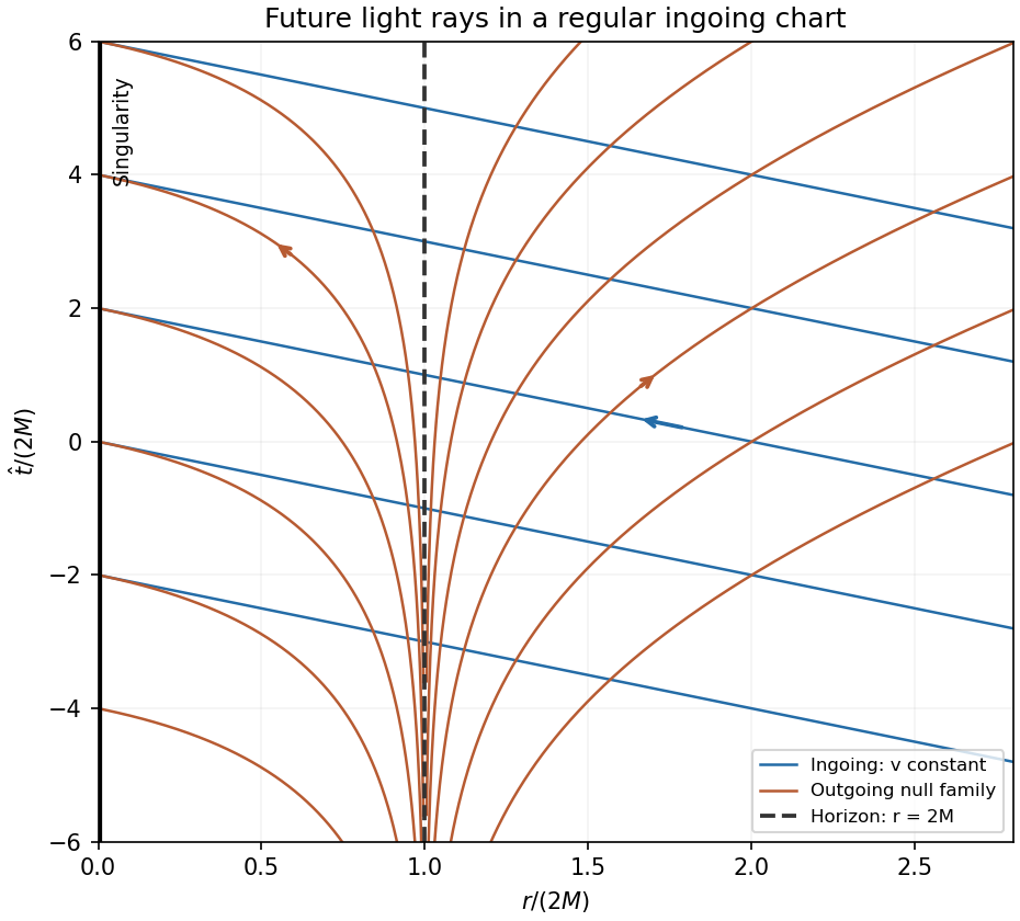
Radial null trajectories in a regular ingoing Schwarzschild chart, with future directions and the event horizon marked
. Details. 
The line is the Schwarzschild event horizon, a null boundary of the future black-hole region. It is a coordinate singularity of Schwarzschild time, not a curvature singularity; the curvature singularity is at . Signals from the future black-hole interior cannot cross it outward.
Finally parametrize any future-directed timelike observer in that interior by proper time . Normalization in the given metric givesThe future direction in the ingoing chart has , so . The proper-time bound inside a Schwarzschild black hole isThus a future-continued observer must reach the singular boundary in finite proper time, regardless of acceleration or angular motion. The black-hole future orientation is essential; a past-directed path or a future path in a white-hole interior is a different statement.
Past exam of the mathematics course of the University of Cambridge 2008 ii Paper 4 35D Solution Created 2026-09-24 Updated 2026-10-14
Use signature , which is required for the stated tensor convention. Then . The time component is , while gives the spatial components . Thus
The scalar is the charge density in the medium's rest frame. In that frame , so and . The rest-frame Ohm's law is precisely their proportionality with rest conductivity . Both sides are four-vectors, so its covariant form isThe time and spatial components respectively giveEliminate to obtainIf the rest-frame charge density vanishes, set , not necessarily in the lab frame. ThenThe induced lab charge is the term that cancels the longitudinal correction in the general formula.
Past exam of the mathematics course of the University of Cambridge 2008 ii Paper 4 34D Solution Created 2026-09-24 Updated 2026-10-14
At zero temperature, fill all momentum states inside the Fermi sphere, with two spin states per momentum. Phase-space counting givesFor dispersion , the ratio of energy to particle-number integrals isLet be the common chemical potential in the weak field, and let denote the lower Zeeman-energy branch . Its populations areKeeping changes only at order , so to first order it equals . Subtracting the two populations givesEach excess lower-energy spin contributes moment along the field. Hence the Pauli moment of a massless electron gas isThis includes the spin contribution specified in the problem. The field is weak enough that both spin branches remain occupied, and orbital magnetic effects are not part of the assumed energy model.
Past exam of the mathematics course of the University of Cambridge 2008 ii Paper 4 33E Solution Created 2026-09-24 Updated 2026-10-14
A periodic lattice Hamiltonian commutes with lattice translations. The Bloch theorem therefore classifies its states by characters of the translation group:where is lattice periodic. For each crystal momentum , solving on a primitive cell with the corresponding quasiperiodic boundary condition gives discrete eigenvalues indexed by . Their continuous dependence on produces the energy bands as ranges through the Brillouin zone. Bragg mixing opens gaps at suitable degeneracies, although bands can overlap in three dimensions and gaps are not guaranteed between every pair.
The quantum numbers are band index, wavevector modulo reciprocal lattice vectors, and spin where spin is conserved. In a finite crystal the allowed wavevectors are discrete; in the thermodynamic limit they become dense and the band description emerges. Spin-orbit coupling can replace a separately conserved spin label by an appropriate internal band label.
Dilute randomly placed impurities break exact translation symmetry, so crystal momentum is no longer an exact quantum number. Most extended states retain approximately the host band structure but acquire impurity scattering and disorder broadening. An impurity potential can also produce impurity levels in a crystal, often in a band gap: levels associated with a donor impurity lie near the conduction-band edge and can supply electrons, while those associated with an acceptor impurity lie near the valence-band edge and can create holes. The impurity's species and potential determine whether such levels exist and how deep they are; not every impurity necessarily makes a gap state. At low density these levels are nearly isolated, while overlap at increasing density can broaden them into an impurity band. Added or removed carriers shift the chemical potential as well.
Past exam of the mathematics course of the University of Cambridge 2008 ii Paper 4 32D Solution Created 2026-09-24 Updated 2026-10-14
For a time-independent reference Hamiltonian, define interaction-picture states and observables byThe transformation is unitary, so matrix elements and expectation values are unchanged; the two pictures make the same physical predictions. Differentiating the state and using the Schrödinger equation cancels the term and gives the interaction picture evolutionIntegrating once and replacing the evolving state in the integral by its initial state gives . For , the first-order transition amplitude therefore yields
For the oscillator, and . Only neighboring levels have a first-order amplitude. Write . The two phase integrals are and its conjugate, whose squared modulus is . To order ,At resonance take their continuous limits, and . All other distinct-level probabilities vanish to this order. Normalization gives to this order, and the downward probability is zero when .
The allowed transition rate is proportional to , so its central peak has width of order about . Distributionally, . Thus both allowed transitions become sharply resonant at the oscillator frequency. Near the peak, perturbation theory still requires ; its coherent growth cannot be extrapolated indefinitely at fixed coupling.
Past exam of the mathematics course of the University of Cambridge 2008 ii Paper 4 31A Solution Created 2026-09-24 Updated 2026-10-14
Put . Substitute into . The leading coefficient gives , and the next gives . Thus , . The coefficient of then givesIn particular and . The two Bessel inverse-power expansions at infinity start asTheir independent leading oscillations give two independent asymptotic solutions, represented by suitable multiples of and on the positive-real large- sector.
For the Liouville–Green approximation, giveswhere the integration constant is absorbed in the amplitude. Hence its two leading wave forms have first two termsExpanding one order further gives the same as the formal recurrence.
The infinite sums must be interpreted as asymptotic expansions, not literal convergent inverse-power series. For integer , never equals , so the recurrence never truncates, and . Thus the inverse-power series diverges at every finite nonzero . Exact Hankel solutions have these asymptotic series; the printed “solutions of the form” uses that customary asymptotic meaning.
Past exam of the mathematics course of the University of Cambridge 2008 ii Paper 4 30C iv Created 2026-09-24 Updated 2026-09-24
There are unlisted articles, also show them or only show them.