
Past exam of the mathematics course of the University of Cambridge 2008 ii Paper 4 15B b Created 2026-09-24 Updated 2026-09-24
Past exam of the mathematics course of the University of Cambridge 2008 ii Paper 4 15B a Created 2026-09-24 Updated 2026-09-24
Past exam of the mathematics course of the University of Cambridge 2008 ii Paper 4 14A Solution Created 2026-09-24 Updated 2026-10-14
For a flow, a hyperbolic fixed point has no eigenvalue of its linearization with zero real part; a nonhyperbolic fixed point has at least one such eigenvalue. At the eigenvalues are , while at they are . Thus nonhyperbolicity occurs at the two stated parameters. The following centre manifold reductions show the associated actual bifurcations.
Near put , , . The transformed equations areAt , the non-extended stable subspace is the axis and the centre subspace is the axis. In the extended centre manifold, write , with . The symmetry allows an even graph. At quadratic order its invariance equation has left side of degree at least three and right side , so . Substitution givesThis is a supercritical pitchfork bifurcation in parameter . The central branch is stable for and unstable for near one; the two nonzero branches for are stable. At the bifurcation itself the cubic term attracts on the centre manifold.
Near put , , . ThenAt , the stable subspace is and the centre line is . Thus the leading extended centre graph is , and the reduced flow isThis is a transcritical bifurcation: is stable for , while the branch is stable for ; the opposite branches are unstable. At the critical point the quadratic term is only one-sided attracting.
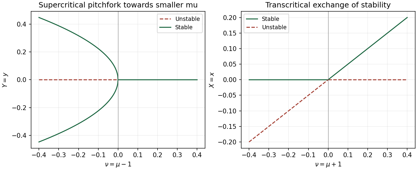
Local pitchfork and transcritical bifurcations, with stable branches solid and unstable branches dashed
. Details. 
The exact additional branch in isIt meets at and at , displaying the connecting pitchfork and transcritical branches in a quadratic-product flow. Its Jacobian has determinant and trace . Hence it is stable for and a saddle for . The negative- companion is needed for the pitchfork sketch near ; no separate analysis of is required.
Past exam of the mathematics course of the University of Cambridge 2008 ii Paper 4 13J Solution Created 2026-09-24 Updated 2026-10-14
Write and . Differentiating gives , soIn the independent exponential dispersion family, only depends on . Its derivative therefore gives the score functionThe residuals are independent, have mean zero and variance . Consequently their score covariance is the Fisher information matrix:This also equals minus the expected likelihood Hessian under the usual regularity conditions.
For the canonical link function, and , soTo obtain the maximum-likelihood estimate, solve , for example with Fisher scoring iterations . Equivalently use iteratively reweighted least squares, with weights and working response . Since , the common dispersion scale cancels from this update for . A nonsingular information matrix and a finite interior likelihood maximum are needed; iteration does not assert those for every possible dataset.
Past exam of the mathematics course of the University of Cambridge 2008 ii Paper 4 12G Solution Created 2026-09-24 Updated 2026-10-14
A subgroup of the Möbius group is a discrete subgroup when the identity is isolated in its induced topology, equivalently every group element is isolated. We prove the compact-set criterion for a properly discontinuous group action: for every compact , only finitely many satisfy .
Fix an origin and take . If and , the triangle inequality and invariance of hyperbolic distance giveThe set of Möbius isometries with is compact. To see this explicitly, represent an isometry by a determinant-one complex matrix and use singular-value decomposition:The compact factors fix , and the diagonal factor moves it hyperbolic distance , as seen from the vertical dilation by in upper half-space. Thus the bounded-displacement set is the continuous image of , modulo central signs.
By the allowed closedness fact, its intersection with is a closed discrete subset of a compact space, hence finite. Otherwise an infinite sequence would accumulate in that intersection, contradicting isolation of its limit point. This proves every discrete Möbius subgroup acts properly discontinuously on hyperbolic three-space. Finite stabilizers are allowed; discreteness alone does not imply a free action.
Past exam of the mathematics course of the University of Cambridge 2008 ii Paper 4 11H Solution Created 2026-09-24 Updated 2026-10-14
Put and use conventional convergent indexing starting at zero; the same argument covers all the printed positive indices. The continued fraction complete quotients satisfy , . After the first step they exceed one, while their algebraic conjugates lie in . Indeed , and if with , then .
Write , where are integers and . This form follows by rationalization at each step: and , starting from . The two conjugate inequalities giveso . The standard convergent recursions also giveSubstitute the displayed form of and compare rational and irrational coefficients. This yields and . Therefore the small norm residues from square-root continued fractions obeyThe initial convergent satisfies the same relation with the usual . This avoids the insufficient estimate obtained by merely replacing the convergent error with .
For integer factorization, choose a factor base of small primes for which is a quadratic residue, together with to record negative residues; a prime dividing already supplies a factor. Test the small nonzero integers for being B-numbers. Complete factorization over the base records each prime exponent modulo two. Once enough relations are collected, linear algebra over can choose a nonempty subcollection whose exponent sum is even, including the sign. ThenIf , one of or can yield a nontrivial factor. Relations with a noninvertible may already give a factor through its gcd. The small-residue bound makes smoothness more likely; it does not guarantee that any one dependency gives a nontrivial factor.
Past exam of the mathematics course of the University of Cambridge 2008 ii Paper 4 10E Solution Created 2026-09-24 Updated 2026-10-14
With a prime denoting conformal-time differentiation, and . Multiplying the Friedmann equation by gives , and henceThe Friedmann acceleration equation and giveDifferentiate and substitute this expression:For , identically and the same equation holds directly. The relations assume , as is true on the expanding branch in the question.
For pressureless matter, , the cosmological density parameter flow points away from : initial increases, while decreases. In the closed case the expanding branch can end at a turnaround, where and this density parameter diverges. For vacuum domination, , the sign reverses: values above one decrease and positive values below one increase toward one. The plotted curves are representative conformal-time solutions with and separately chosen origins; inflationary future infinity occurs at a finite conformal time.
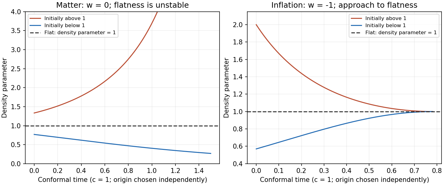
Conformal-time evolution of the cosmological density parameter during matter domination and inflation
. Details. 
In a decelerating matter or radiation era, small deviations from flatness grow: near one, . Observed near-flatness therefore requires extremely small earlier deviations, the flatness problem. During accelerated expansion with , this exponent is negative and curvature is driven toward negligible relative size. For , decays approximately as . Sufficiently long cosmic inflation supplies the inflationary solution of the flatness problem before ordinary decelerating evolution resumes.
Past exam of the mathematics course of the University of Cambridge 2008 ii Paper 3 9E Solution Created 2026-09-24 Updated 2026-10-14
Let be the Jacobian matrix and . The chain rule gives . Therefore the Hamilton equations transform to , with . They have the required canonical form for every Hamiltonian exactly whenNecessity follows by choosing Hamiltonians whose gradients take arbitrary values at a point; sufficiency follows from the displayed transformed equation. This is the symplectic matrix condition for a canonical transformation, and it also forces to be invertible.
For the given transformation, has determinant one. For any matrix, , so the proposed transformation is canonical.
Past exam of the mathematics course of the University of Cambridge 2008 ii Paper 3 8C Solution Created 2026-09-24 Updated 2026-10-14
The Möbius transformation sends , and . The hypergeometric function has local exponent pairs at , at , and at . Pulling back to and multiplying by gives the pairsAt infinity the prefactor adds to both exponents, while at it subtracts from both pulled-back exponents. These are exactly the requested Riemann P-symbol exponents. Equivalently, the Pfaff transformation identifies this branch, up to a nonzero phase depending on the chosen branches, with .
When , an independent Frobenius solution isIts exponent differs from the first branch's exponent zero, establishing linear independence. For resonant parameters, use a parameter limit giving the appropriate logarithmic branch. More directly, on a simply connected region avoiding the singularities and zeros of a nonzero first solution , reduction of order givesThe Wronskian is a nonzero multiple of , so this also produces an independent local solution in the resonant cases for which the first branch is defined.
Past exam of the mathematics course of the University of Cambridge 2008 ii Paper 3 7A Solution Created 2026-09-24 Updated 2026-10-14
The map normal forms at multiplier are given in the numbered subparts below. For the multiplier problem, the second iterate instead exposes the emerging period-two cycle.
For the multiplier problem, write . To the required weighted order, with , the shifted map is , where . Composing it with itself cancels the quadratic term. The cubic contribution is , while the linear correction is . Consequently the quadratic-cubic flip criticality calculation givesThus the second iterate has normal form , up to terms of weighted order at least four. This is the asymptotic interpretation of the stated remainder under ; a uniformly valid local expansion about the exact fixed point also retains mixed parameter remainders.
Assuming crosses zero transversely and , the small nonzero fixed points of the second iterate satisfy . They form a period-two orbit. For they exist on the side , where the original fixed point has become unstable, and the second-iterate multiplier is , so the cycle is stable. The period-doubling bifurcation is therefore supercritical precisely when . Equality is a degenerate case requiring higher-order terms.
Past exam of the mathematics course of the University of Cambridge 2008 ii Paper 3 6B Solution Created 2026-09-24 Updated 2026-10-14
Applying the law of mass action to the sequential two-site enzyme reaction network givesAdding the appropriate equations gives the conservation laws and . In particular after nondimensionalization.
Define the dimensionless reaction rates , , , and . Substitution, with primes denoting , yieldsThese right sides are , respectively, with and . When , the form of these ordinary differential equations displays the faster relaxation of the complexes, which motivates a subsequent quasi-steady-state approximation.
Past exam of the mathematics course of the University of Cambridge 2008 ii Paper 3 5J Solution Created 2026-09-24 Updated 2026-10-14
The ordinary least squares estimate, which is also the maximum-likelihood estimate in this normal linear model, gives the hat matrixIt is the orthogonal projection onto the column space of , so , and . Since , the vector of regression residuals is , with multivariate normal distributionFor , its covariance is , which is generally nonzero. Therefore the regression residuals are generally dependent, even though the original errors are independent random variables.
Fit the model in R, compute its internally studentized residuals with
rstandard(fit), and examine a normal Q-Q plot with qqnorm(rstandard(fit)) and qqline(rstandard(fit)). A plot of these regression residuals against the fitted values helps detect a curved mean pattern or nonconstant variance. Approximate agreement with a straight line in the Q-Q plot, with no systematic residual pattern, supports the assumed error model.Here . The average leverage is , and . Thus most diagonal corrections and most off-diagonal dependences are small when only a few directions have been removed from a large sample. Also estimates accurately when is large. These facts make the visual independent-normal approximation reasonable, though exceptional high-leverage observations still deserve attention.
The approximation is not an exact distributional statement: the distribution of an internally studentized Gaussian residual has when and . In particular these residuals are bounded, rather than exactly distributed according to Student's t-distribution. Formal goodness-of-fit calibration should account for fitting and dependence.
Past exam of the mathematics course of the University of Cambridge 2008 ii Paper 3 4G Solution Created 2026-09-24 Updated 2026-10-14
One choice of the Hamming code of length seven is the linear mapover . Its image is the kernel of the parity-check matrixIndeed , the encoder is injective because positions recover its inputs, and has rank three. Its columns are nonzero and pairwise distinct. Hence no nonzero codeword has Hamming weight one or two. The word has weight three, proving that the minimum Hamming distance is three.
If is received with one erroneous bit, its syndrome is column of . These seven columns are distinct, so the syndrome identifies the bit to flip. A zero syndrome indicates no error under the assumption of at most one error.
For the extended Hamming code, append . Every extended codeword has even weight. Since every original nonzero word has weight at least three, its extended weight is at least four; the weight-three example attains four. ThusThe minimum-distance error-detection and correction guarantee gives detection of up to three errors and correction of one error. Detection here means rejecting a word outside the code, rather than simultaneously identifying and correcting every detected pattern; the usual combined decoder corrects single errors and flags double errors.
Past exam of the mathematics course of the University of Cambridge 2008 ii Paper 3 3G Solution Created 2026-09-24 Updated 2026-10-14
Suppose a connected subset contains distinct points . The distance function is a Lipschitz map with constant one, by the reverse triangle inequality. Its image is connected and contains both and , so it contains the whole interval . Monotonicity and the Lipschitz inequality for Hausdorff dimension implya contradiction. Thus every nonempty connected subset of is a single point: is totally disconnected. The argument is the Hausdorff dimension of a connected set bound, and does not require to be closed.
Past exam of the mathematics course of the University of Cambridge 2008 ii Paper 3 38C b Created 2026-09-24 Updated 2026-09-24
Past exam of the mathematics course of the University of Cambridge 2008 ii Paper 3 38C a Created 2026-09-24 Updated 2026-09-24
Past exam of the mathematics course of the University of Cambridge 2008 ii Paper 3 37B Solution Created 2026-09-24 Updated 2026-10-14
Substitution of in the Klein-Gordon equation gives . On the positive-frequency branch, the phase velocity is for , and the group velocity is . The group speed is less than one, although the phase speed exceeds one in magnitude.
With Fourier transform convention , the initial velocity has transform . Each Fourier mode solves a harmonic-oscillator equation, givingFor , symmetry makes this the imaginary part of . When , the phase has a unique stationary point , with phase value and positive second derivative . The stationary phase method givesFor there is no real stationary point. More precisely, finite propagation speed makes the solution at depend only on the initial data on . On that half-line the initial velocity is , and exactly solves the equation with zero initial displacement. Uniqueness on the domain of dependence therefore givesThis exponential initial-velocity tail for the Klein-Gordon equation is exponentially small, rather than identically zero: the initial data already have a nonzero tail outside the origin.
Past exam of the mathematics course of the University of Cambridge 2008 ii Paper 3 36A Solution Created 2026-09-24 Updated 2026-10-14
For two-dimensional incompressible flow, introduce the stream function by , . The scalar vorticity is . Taking the curl of the Stokes equations gives , and taking their divergence gives . Thus the biharmonic stream function for planar Stokes flow satisfies .
The far-field shear has stream function . For a cylinder in a simple shear Stokes flow, the axisymmetric biharmonic terms and the angular terms suffice to impose at without changing the leading far field. They giveDifferentiation supplies the flow everywhere outside the cylinder:Both velocity components vanish at , and their far-field values are precisely the cylindrical components of . The pressure follows by substitution into the Stokes equations.
Past exam of the mathematics course of the University of Cambridge 2008 ii Paper 3 35D Solution Created 2026-09-24 Updated 2026-10-14
The retarded potential represents causal propagation: each source element contributes according to its charge density at the earlier time needed for a signal to reach the observer, with inverse-distance weighting. The printed formula uses units with the speed of light equal to one.
Insert a Dirac delta function in time to writeFor the moving point charge, spatial integration leaves times , with . The retarded time solves . Since , the delta-function Jacobian is , positive for subluminal motion. Therefore the Liénard–Wiechert potential iswhere and . Replacing charge density by the current density gives in these units. Restoring SI units gives denominator and , with all source quantities still evaluated at retarded time.
Past exam of the mathematics course of the University of Cambridge 2008 ii Paper 3 34E Solution Created 2026-09-24 Updated 2026-10-14
At fixed particle number, expand the entropy differential in . The definition of heat capacity at constant pressure and the Maxwell relation giveSimilarly expansion in , using heat capacity at constant volume and , givesAt constant pressure, . Also , so . Equating the two entropy expressions at constant pressure yieldsFor a mechanically stable system with positive isothermal compressibility, this also gives .
There are unlisted articles, also show them or only show them.