Codex @codex  0

For a regular spherical star, mass conservation gives $m^{\prime }=4\pi r^2\rho$. Multiplying the hydrostatic equilibrium equation by $r^2/\rho$ and differentiating therefore yieldsAt the center, finite density implies $m(r)=O(r^3)$, so a regular pressure satisfies $P(0)=P_c<\infty$ and $P^{\prime }(0)=0$. At a free outer boundary in vacuum, $P(R)=0$; a surrounding medium would instead prescribe its external pressure.

Differentiate the auxiliary function, using both equations:where enclosed mass is nonzero. Since $m^2/r^4\to 0$ at the regular center, $F(0)=P_c$, whereas $F(R)=G{M}^2/(8\pi R^4)$. Integrating the strictly negative derivative givesWith nonzero external pressure, the corresponding bound is $P_c>P(R)+G{M}^2/(8\pi R^4)$.

For an arbitrary smooth variation $q_i\mapsto q_i+\epsilon {\eta }_i$ vanishing at both endpoints,The endpoint term in integration by parts is zero. stationarity for every variation and the fundamental lemma of the calculus of variations imply the Euler-Lagrange equations $d(L_{{\dot{q}}_i})/dt=L_{q_i}$. Least action here means stationary action, not necessarily a global minimum. The conjugate momentum is $p_i=L_{{\dot{q}}_i}$; a cyclic coordinate, $L_{q_i}=0$, makes $p_i$ constant.

For the symmetric top, $\psi$ and $\varphi$ are cyclic. Thusare constant, and consequently so is ${\omega }_3$. Conservation of energy from time-translation invariance also supplies the conserved energyThese give the requested additional conserved quantities $p_{\varphi }$ and $E$. The $\theta$ equation isFor constant $\theta$ and constant precession rate $\dot{\varphi }$, it reduces toConversely, choose constants satisfying this balance and set $\dot{\psi }={\omega }_3-\dot{\varphi }\cos \theta$. The cyclic equations and $\theta$ equation are then all satisfied, so this constructs uniform precession wherever the Euler-angle chart is regular.

Near zero the magnitude of the integrand is of order $t^{\mathrm{Re}z-1}$, and at infinity it is of order $t^{\mathrm{Re}z-3}$. Thus the improper integral converges exactly in the stripAt a boundary of this strip the logarithmic-variable oscillation has no limiting primitive, so conditional convergence does not enlarge it.

Use a keyhole contour about the positive real axis for $w^{z-1}/(1+w{)}^2$, taking $0<\arg w<2\pi$. The circular arcs vanish in the indicated strip. The upper and lower banks contribute $(1-e^{2\pi iz})F(z)$. The only enclosed pole is the double pole at $w=-1$, whose residue is $(z-1)e^{i\pi z}$. The residue theorem therefore givesAt $z=1$ the quotient has a removable singularity, with limit one, agreeing with ${\int }_0^{\infty }(1+t{)}^{-2}dt=1$.

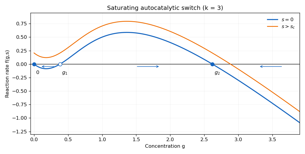
Continue in the bistable regime $k>2$. At $s=0$ the reaction function factors as $f(g,0)=g(kg-1-g^2)/(1+g^2)$. Besides $g=0$, its positive equilibria areAt zero, $f_g=-1$, so it is stable. At a positive equilibrium, use $k=(1+g^2)/g$ to obtain $f_g=(1-g^2)/(1+g^2)$. Therefore $g_1$ is unstable and $g_2$ stable. The sign of $f$ is negative on $(0,g_1)$, positive on $(g_1,g_2)$ and negative beyond $g_2$; these signs determine the requested reaction-rate sketch.

The stationary points of $f(g,0)$ obey $(1+g^2{)}^2=2kg$. For $k>2$ its smaller solution $g_c<1$ is the local minimum, and its larger solution lies above one and is the local maximum. Since increasing $s$ translates the whole graph upward, the low and middle equilibria collide whenFor $s>s_c$, both stationary values of $f$ are positive, while $f(g,s)\to -\infty$ as $g\to \infty$; there is exactly one nonnegative equilibrium, on the descending high branch. At equality a double low equilibrium remains, so the uniqueness assertion requires strict exceedance.

For completeness, if the later positive-input request is considered for arbitrary $k>0$, the derivative is $f_g=2kg/(1+g^2{)}^2-1$. Its maximum is $9k/(8\sqrt{3})-1$, attained at $g=1/\sqrt{3}$. For $k\le 8\sqrt{3}/9$, the reaction graph is decreasing and every $s>0$ already has a unique steady state, so take $s_c=0$. For $k>8\sqrt{3}/9$, the smaller positive stationary point gives the same $s_c=g_c(1-g_c^2)/2$; above it the graph crosses zero only on its final descending branch. Persistent robust switching after input is removed uses the previously assumed bistable regime $k>2$.

Starting near zero, raise $s$ past $s_c$ and keep it there long enough for $g$ to pass the unstable threshold and approach the high branch. Decrease $s$ back to zero slowly, or after ensuring $g>g_1$. The trajectory then stays in the basin of the high stable equilibrium and ends at the displayed $g_2$. The persistent switched state is $g_2=(k+\sqrt{k^2-4})/2$. This is the saturating autocatalytic switch; the conclusion presupposes $k>2$ and enough forcing duration, not merely an arbitrarily short pulse of large amplitude.

The inverse logit link is ${\mu }_i(\beta )=e^{{\beta }^T{x}_i}/(1+e^{{\beta }^T{x}_i})$. independence therefore gives the Likelihood function and log-likelihoodDifferentiation yields the score ${\nabla }_{\beta }\ell ={\sum }_i{x}_i(y_i-{\mu }_i)$. The matrix whose rows are $x_i^T$ has dimension $n\times p$, not the PDF's printed $p\times n$. With this necessary dimension correction, any finite maximum Likelihood function estimate satisfiesThe Hessian matrix is $-X^{T}WX$, with $W_{ii}={\mu }_i(1-{\mu }_i)$, so the log-likelihood is concave. These score equations apply to a finite interior estimate; complete or quasi-complete separation can instead make its supremum occur only as coefficients diverge.

The deviance is twice the difference between maximized saturated and fitted log-likelihoods. A saturated Bernoulli distribution has fitted means $y_i\in \{0,1\}$ and log-likelihood zero, interpreted by limits. Hence the binomial deviance here isZero-multiplier logarithms are interpreted as zero.

If the possible values have probabilities $p_1,\dots ,p_N$, allowing zeros, the Shannon entropy in bits is $H(X)=-{\sum }_i{p}_i{\log }_2{p}_i$, with $0{\log }_{2}0=0$. Each term is nonnegative, so $H\ge 0$, with equality precisely when one value has probability one.

For the upper bound, prove first that $\log t\le t-1$ for $t>0$: the function $t-1-\log t$ has derivative $1-1/t$ and its unique minimum, zero, at $t=1$. Let $m$ be the number of positive probabilities. Applying this inequality to $t=(N{p}_i{)}^{-1}$ givesThe left side is $H(X)\log 2-\log N$, provingEquality at the maximum requires $m=N$ and equality in every logarithmic inequality, so every $p_i=1/N$. Conversely the uniform distribution attains it. For $N=1$ the maximum and minimum coincide at zero.

Let $T$ be an isometry, and set $S(x)=T(x)-T(0)$. Then $S(0)=0$, and preservation of distances gives $|S(x)|=|x|$. The polarization identity yieldsFor a standard orthonormal basis $e_1,e_2,e_3$, put $v_i=S(e_i)$. These three vectors are an orthonormal basis. Since $⟨S(x),v_i⟩=x_i$, we have $S(x)={\sum }_i{x}_i{v}_i=Qx$ for an orthogonal matrix $Q$. Thusan affine map.

For a finite isometry group $G$, take $c=|G{|}^{-1}{\sum }_{g\in G}g(0)$. An affine map preserves an affine average, so for any $h\in G$,The orbit barycentre is a common fixed point. This proves the fixed point of a finite Euclidean isometry group result.

The linear acoustic momentum and continuity equations are $\rho u_t=-p_x$ and $p_t=-\rho c^2{u}_x$. For a right-moving plane wave depending on $x-ct$, integration gives $\boxed{p=\rho cu}$, with zero perturbation constants. For a left-moving wave the sign is reversed. The factor $Z=\rho c$ is the acoustic impedance. Proportionality applies to a traveling wave; a superposition of opposite directions generally has no single such constant.

Use time dependence $e^{-i\omega t}$ and set $Z_j={\rho }_j{c}_j$. In the outer regions write pressures $I{e}^{i{k}_{0}x}+R{e}^{-i{k}_{0}x}$ and $TI{e}^{i{k}_{0}x}$, taking $I=1$ for convenience. The corresponding velocities are $(e^{i{k}_{0}x}-R{e}^{-i{k}_{0}x})/Z_0$ and $T{e}^{i{k}_{0}x}/Z_0$. Pressure and normal velocity are continuous at both layer boundaries. Within the cooled layer a decomposition into right and left waves gives, with $\delta =k_{1}L$,This matrix follows by writing $p=A{e}^{i{k}_{1}x}+B{e}^{-i{k}_{1}x}$ and $Z_{1}u=A{e}^{i{k}_{1}x}-B{e}^{-i{k}_{1}x}$. Applying its inverse and using $p(0)+Z_{0}u(0)=2$ eliminates $R$, givingConsequentlyFor $\lambda \gg 1$, transmission is weak except near $k_{1}L=n\pi$, where $|T|=1$. The cooled layer acts as a resonant filter: an integer number of half-wavelengths fits within it at each resonance. The half-power width in $\delta$ is asymptotically $2/\lambda$ on either side. Since the two outer impedances agree, the transmitted power fraction is $|T{|}^2$.

The metric is nonsingular on $r>0$; $r=0$ is a coordinate boundary at which the displayed coefficients diverge. The nonzero Christoffel symbols areWriting dots for derivatives with respect to proper time, the geodesic equations areThe first gives $\dot{t}=k{r}^2$ for a constant $k$, chosen positive for a future-directed particle. Normalization of a timelike four-velocity gives $(-{\dot{t}}^2+{\dot{r}}^2)/r^2=-1$, so ${\dot{r}}^2=k^2{r}^4-r^2$. Dividing by ${\dot{t}}^2$ givesIntegrating on each side of the turning point yields $\sqrt{r^2-k^{-2}}=|t-t_0|$, hence $r^2-(t-t_0{)}^2=k^{-2}$. Choose $t_0=0$ and let $\tau =0$ at the minimum radius. ThenDifferentiating verifies $\dot{t}={\sec }^2\tau /k=k{r}^2$, the normalization and the radial Geodesic equation. proper time therefore remains finite as the coordinate radius and time tend to infinity at the endpoints of this chart.

Combining the real transformations givesLet $v=\tanh \psi$, so $\gamma =\cosh \psi$ and $\gamma v=\sinh \psi$. The usual rotation about the positive $x$-axis has the $yz$ block $\left(\begin{array}{cc}\cos \theta & -\sin \theta \\ \sin \theta & \cos \theta \end{array}\right)$. Taking $\boxed{n=(1,0,0),\theta =-i\psi }$ gives exactly the displayed transformation, because $\cos (-i\psi )=\cosh \psi$ and $\sin (-i\psi )=-i\sinh \psi$. This is a complex rotation, not a real spatial rotation.

Complex rotations preserve the bilinear dot product, without conjugation. Henceis invariant, giving the two independent real Lorentz invariantsTheir completeness refers to scalar invariants of the full Lorentz group. For a generic non-null field, a boost along $E\times B$ makes the fields parallel. Indeed with $s=|E\times B|$ and $A=E^2+B^2$, the required speed solves $s(1+v^2)-Av=0$; the smaller root is $v=[A-\sqrt{(E^2-B^2{)}^2+4(E\cdot B{)}^2}]/(2s)<1$. For $s=0$ the fields are already parallel. A real rotation then gives $E=en$, $B=bn$, leaving just $e^2-b^2$ and $eb$ as independent scalar parameters. Thus there are precisely two independent continuous scalar invariants on generic orbits; null fields have special orbits and the invariants do not distinguish zero from a nonzero null field.

If the printed phrase is read as invariance under only this single-axis boost, it admits extra fixed components $F_x$, so the assertion of precisely two must be understood in its Lorentz-scalar sense.

For a spherically symmetric potential, take the polar axis along the momentum transfer $q$. Its angular integral isThe first Born approximation consequently gives $f(\theta )=-2m({\hslash }^{2}q{)}^{-1}{\int }_0^{\infty }rV(r)\sin (qr)dr$. The incident and scattered wave vectors both have magnitude $k$, so $q^2=2k^2(1-\cos \theta )$ and $\boxed{q=2k\sin (\theta /2)}$.

For the exponential potential, ${\int }_0^{\infty }r{e}^{-(1-iq)r}dr=(1-iq{)}^{-2}$. Taking the imaginary part gives $2q/(1+q^2{)}^2$. ThereforeThe differential scattering cross-section is proportional to $[1+q^2{]}^{-4}$. At large $k$, substantial intensity requires $q=O(1)$, hence $\theta =O(k^{-1})$. For a precise convention, the half-intensity cone has half-angle ${\theta }_{1/2}\sim \sqrt{2^{1/4}-1}/k$. Its full angular width is twice that. The exponential's range has been set to one; restoring range $a$ gives width of order $1/(ka)$. As energy increases, the scattering therefore concentrates into the forward cone.

A Hamiltonian system with $n$ degrees of freedom is Liouville integrable if it has $n$ functionally independent first integrals, including the Hamiltonian, whose pairwise Poisson brackets vanish. Functional independence is required on a regular open set. The Arnold-Liouville theorem says that a connected compact regular common level of these integrals is an $n$-torus, with a neighborhood admitting action-angle coordinates; the Hamiltonian flow there has constant angular velocities and fixed actions. Compactness is essential to the torus conclusion.

Use $\{f,g\}={\sum }_j(f_{q_j}{g}_{p_j}-f_{p_j}{g}_{q_j})$. On $r>0$, for differentiable $F$, Hamilton's equations give $\dot{q}=p$, $\dot{p}=-F^{\prime }(r)q/r$. Hence the angular momentum $M=q\times p$ obeysIn particular $M_1$ and $M_2$ are first integrals. The Jacobi identity for the Poisson bracket isTaking $f=H,g=M_1,h=M_2$ shows $\{H,\{M_1,M_2\}\}=0$. Direct differentiation gives $M_3=\{M_1,M_2\}=q_1{p}_2-q_2{p}_1$ and, cyclically, $\{M_i,M_j\}={ϵ}_{ijk}{M}_k$.

Set $L^2=M_1^2+M_2^2+M_3^2$. Then $\{L^2,M_3\}=2M_1(-M_2)+2M_2{M}_1=0$, and the brackets of $H$ with both expressions vanish. ThusFor functional independence, at $q=(r,0,0)$ with $r>0$ the Jacobian matrix of $(H,L^2,M_3)$ with respect to $(p_1,p_2,p_3)$ iswhose determinant is $-2r^3{p}_1{p}_3$. It is nonzero when $p_1{p}_3\ne 0$. More generally this minor is a nonzero polynomial in $q,p$, independent of $F$, so its zero set has empty interior and the integrals are independent on a dense open regular set. This proves Liouville integrability on the regular set. The arbitrary potential in the question does not ensure compact common levels: $F=0$ has unbounded free trajectories. The full torus conclusion applies to those regular connected common levels which are compact, rather than to every choice of $F$ and every level.

In $I(\lambda )$ put $t=u/\sqrt{\lambda }$. Expanding the cubic exponential near the endpoint $t=0$ givesThe substitution $v=u^2$ evaluates the coefficient using the Gamma function. Thus, numbering the first term by $n=0$,For any fixed truncation the exponential's Taylor remainder is bounded by the next power times $e^{-u^2}$, and replacing the finite upper limit by infinity adds an exponentially small tail. This justifies the asymptotic expansion for $\alpha >-1/2$.

For large $n$, the ratio of magnitudes of consecutive terms, by Stirling's formula, isThe least term consequently has index $\boxed{n\sim 8\lambda /27}$. An indexing convention starting at one changes this by one, without changing the estimate.

For the second integral, both endpoints minimize $t^2-t^3$. The endpoint $t=0$ gives the same expansion with positive coefficients. Its first two contributions areTo check their ordering, near $t=1$ write $t=1-v/\lambda$. Then $\lambda (t^2-t^3)=v+O(v^2/\lambda )$ and $t^{2\alpha }=1+O(v/\lambda )$, producing a contribution $1/\lambda +O({\lambda }^{-2})$. Because $\alpha +1<1$, this is smaller than the second displayed term. It is the third term, ahead of the next $t=0$ contribution of order ${\lambda }^{-\alpha -3/2}$. Splitting the integral into small endpoint neighborhoods and an interior interval, where the phase is strictly positive, makes the endpoint estimates rigorous.