
Past exam of the mathematics course of the University of Cambridge 2008 ii Paper 3 10E Solution Created 2026-09-24 Updated 2026-10-20
Write the photon energy density as , where by the Stefan–Boltzmann law. The photon gas has pressure and zero photon chemical potential. The first law of thermodynamics therefore givesDividing by and integrating gives the entropy density of a photon gas:The integration constant is fixed to zero at zero temperature, consistently with the third law of thermodynamics.
The inequality says interactions act much faster than the expansion time, maintaining local thermal equilibrium. For adiabatic reversible expansion with no additional source of entropy, cosmological entropy conservation fixes the entropy in a comoving volume. Since that volume scales as , and the relativistic degrees of freedom are fixed here, is constant. ThusDuring radiation domination, the Friedmann equation gives , and hence . Fast interactions alone would not exclude an additional entropy-producing process; changing relativistic species likewise changes the simple temperature scaling.
Past exam of the mathematics course of the University of Cambridge 2008 ii Paper 2 9A Solution Created 2026-09-24 Updated 2026-10-14
Varying the Lagrangian gives, with the cyclic angle conventions,All successive angular gaps are in equilibrium, so their two contributions cancel. Because the potential depends only on gaps, a uniform change of all angles costs no energy. Its Hessian therefore annihilates , giving a zero-frequency normal mode. The corresponding motion is rigid rotation, , including a constant common angular shift.
For two particles write . Both cyclic gaps contribute, so the quadratic potential is . With the specified masses, the mass matrix is and the stiffness matrix is . The generalized eigenvalue problem givesThe finite-frequency normal mode keeps the mass-weighted mean angle fixed and changes the angular separation sinusoidally. Together with the two rigid-rotation constants, it spans all small motions about equilibrium.
Past exam of the mathematics course of the University of Cambridge 2008 ii Paper 2 8C Solution Created 2026-09-24 Updated 2026-10-14
For the beta function, split inside the integral to obtain . Integrating the derivative of over gives , since both endpoint terms vanish in the initial domain. Combining these identities yieldsRepeatedly apply this recurrence until . Each resulting expression agrees with the original integral on overlap, so it gives its unique analytic continuation. Possible singularities are only .
Near , . Continuing the recurrence downwards giveswhere the empty product is . The recurrence shows that each singularity is at most a simple pole. If is not a positive integer, all these residues are nonzero and all the listed points are poles. If is a positive integer, poles occur only for ; the later candidates are removable, as is also clear from . This qualification matters when claiming a pole at every nonpositive integer.
Past exam of the mathematics course of the University of Cambridge 2008 ii Paper 2 7A Solution Created 2026-09-24 Updated 2026-10-14
At a stationary bifurcation, a real eigenvalue of the equilibrium linearization crosses zero; the critical motion has zero frequency. At a Hopf bifurcation, a conjugate pair crosses the imaginary axis at with , permitting a nearby limit cycle.
The Hopf normal form has a small cycle when . Its radial multiplier exponent is , while the origin's radial exponent is . Thus: for , there is an attracting spiral and no small cycle; for , a repelling spiral is surrounded by an attracting cycle; for , an attracting spiral is surrounded by a repelling cycle; for , there is a repelling spiral and no small cycle. Outside the repelling cycle in the third case the local radial flow points outward; a cubic normal form makes no global prediction about where it goes.
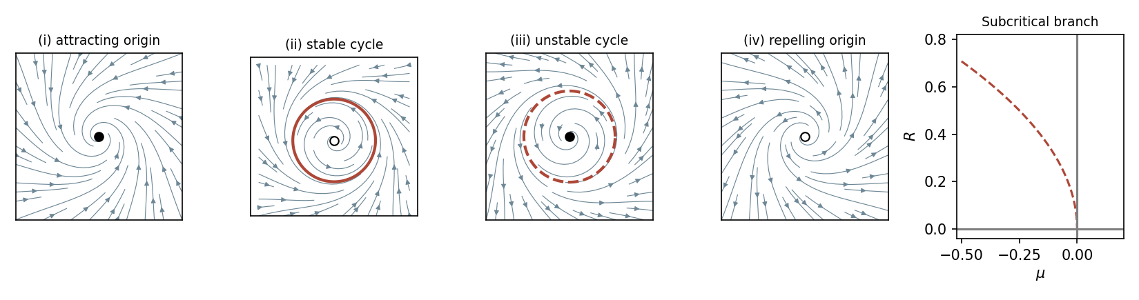
Four local Hopf phase portraits and the unstable subcritical radius branch
. Details. The subcritical bifurcation has and the unstable radius branch on , meeting the origin at . On either existing branch, the angular speed is , so
Past exam of the mathematics course of the University of Cambridge 2008 ii Paper 2 6B Solution Created 2026-09-24 Updated 2026-10-14
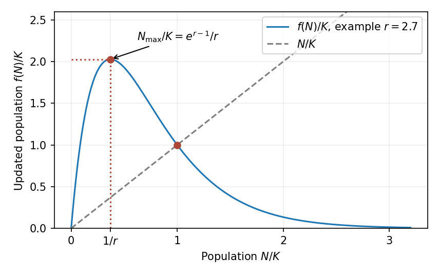
The Ricker population map has equilibria and . Since , their linearization multipliers areThus extinction is unstable and the positive equilibrium is locally asymptotically stable for , becoming unstable for .
To verify an actual period-doubling bifurcation, rather than only a multiplier crossing, put and . The centered map isIts second iterate minus is to leading order. After rescaling , the limiting nonzero roots are simple, so the implicit function theorem continues them. Besides , two nearby points therefore appear for , with . The map exchanges these points, and the derivative of its second iterate there is , so the emerging two-cycle is attracting. The bifurcation at is supercritical period doubling.
For nonnegative populations, increases up to and decreases thereafter to zero. Hence every update after the initial time satisfiesThe bound is attained by choosing ; it is not a bound on an arbitrary initial population.
Past exam of the mathematics course of the University of Cambridge 2008 ii Paper 2 5J Solution Created 2026-09-24 Updated 2026-10-14
Under independent normal distributions, maximum likelihood estimation minimizes subject to . A Lagrange multiplier gives the same correction at every corner. Writing , the interior estimates areThe result is unchanged if the common variance is unknown, since profiling it still minimizes the residual sum of squares. If physical positivity of the three angles is imposed and this projection gives a negative component, the constrained estimate over the closed simplex is instead , with chosen to make the components sum to . If only strictly nondegenerate triangles are admitted, a boundary optimum is merely an unattained likelihood supremum.
The normal-error model is a useful small-error approximation, but its unbounded tails assign positive probability to impossible measured angles. Periodicity or a measurement convention may matter for large errors, and equal variance and independence require experimental justification. The exact sum constraint on the true angles does not itself invalidate independence of three raw measurement errors. After imposing that constraint, however, the fitted-angle errors are correlated: the covariance of the interior estimator is .
Past exam of the mathematics course of the University of Cambridge 2008 ii Paper 2 4G Solution Created 2026-09-24 Updated 2026-10-14
For Shannon-Fano coding, order the symbols by decreasing probability and recursively split each current list into two contiguous groups with total probabilities as close as possible. Label the two branches and ; the path to a symbol is its prefix code word. Here the first split is of weight against of weight . The latter splits into and , each of weight . One answer isFor Huffman coding, repeatedly merge the two least-probable nodes and then read the resulting binary tree from the root. Merge to weight , merge this node with to weight , and merge with . The same displayed prefix code results. Its mean length is . Choices at ties and exchange of binary labels yield other equivalent codes. Huffman coding minimizes mean length among binary prefix codes; the top-down Shannon-Fano construction does not have that general optimality guarantee.
Past exam of the mathematics course of the University of Cambridge 2008 ii Paper 2 3G Solution Created 2026-09-24 Updated 2026-10-14
Every discrete additive subgroup of has the form for linearly independent vectors, with or . A full translation lattice has , and conversely every such integer span is a discrete cocompact subgroup. This classifies planar lattices up to a choice of basis.
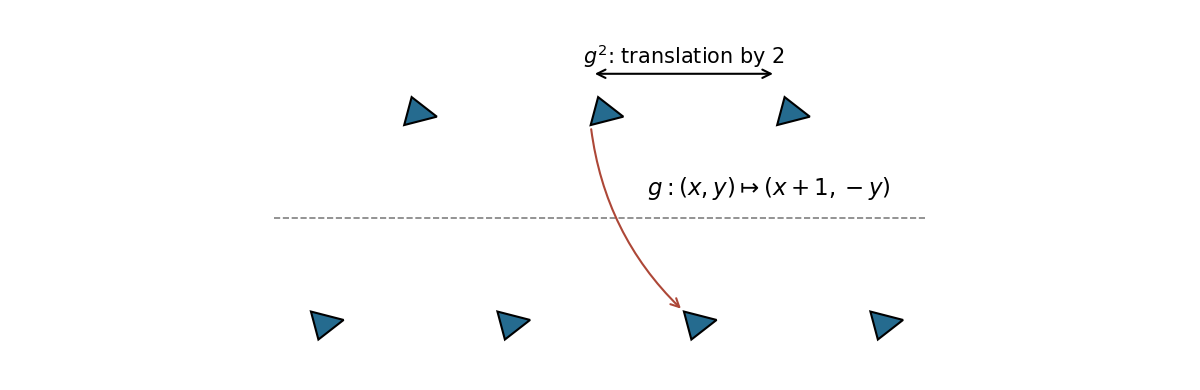
A frieze group is a discrete group of planar Euclidean isometries whose translation subgroup is infinite cyclic and has finite index. Consider the glide reflection . Its square is translation by , whereas every odd power reverses orientation. Therefore , but none of its translation elements generates the whole group: they form the index-two subgroup .
To realize exactly this frieze group, repeat a small scalene triangular motif at the points , reflecting the motif when is odd. Choose the motif with three distinct side lengths and no internal symmetry. The displayed pattern has glide reflection symmetry and translation period , but no pure horizontal reflection or vertical mirror. Distinct side lengths force any symmetry to preserve corresponding vertices, which rules out extra motif permutations; the sequence of heights then leaves exactly the powers of .


Past exam of the mathematics course of the University of Cambridge 2008 ii Paper 2 38C b Created 2026-09-24 Updated 2026-09-24
Past exam of the mathematics course of the University of Cambridge 2008 ii Paper 2 38C a Created 2026-09-24 Updated 2026-09-24
Past exam of the mathematics course of the University of Cambridge 2008 ii Paper 2 37B Solution Created 2026-09-24 Updated 2026-10-14
For isentropic flow of a perfect gas, with and . The mass and momentum equations implyAdding and subtracting the appropriate multiples therefore provesThese are the Riemann invariants for one-dimensional isentropic flow.
In the piston-driven rarefaction wave, the incoming minus invariant has its initial value zero. Thus . At the piston , giving . A plus characteristic emitted at time has constant and , so its straight trajectory isThe first characteristic is , ahead of which the gas is undisturbed. Later characteristics have decreasing propagation speed and spread into a rarefaction. More explicitly for , with equality only at the vacuum endpoint. They never intersect, so no compressive shock forms.
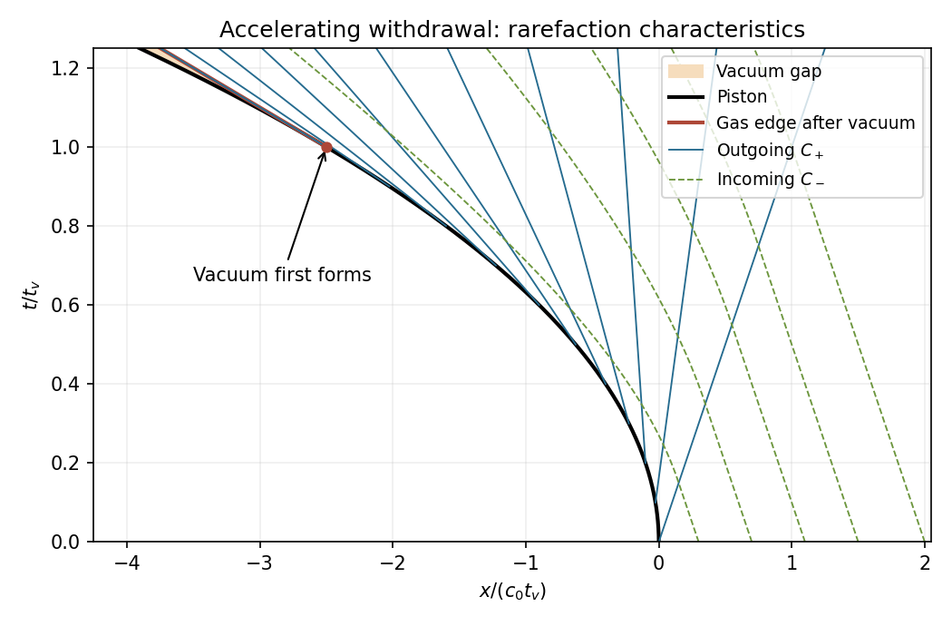
Withdrawing piston, outgoing rarefaction characteristics, incoming characteristics and the vacuum gap
. Details. 
Since , the vacuum formation at an accelerating withdrawing piston givesAt , density, sound speed and pressure at the gas edge vanish, and the piston velocity is . Its speed is the positive magnitude . Afterwards the gas edge continues at this limiting velocity, while the piston keeps accelerating away; a vacuum gap of width opens and the gas pressure on the piston stays zero.
Past exam of the mathematics course of the University of Cambridge 2008 ii Paper 2 36A Solution Created 2026-09-24 Updated 2026-10-14
The lubrication approximation requires depth small compared with the horizontal variation scale , small bottom slopes, and negligible inertia on the scale . Treat the prescribed flat surface as steady and impermeable to leading order. The leading Stokes equations give and . No slip at and the imposed shear yieldIntegration and depth-integrated incompressibility now giveThe surface value is . Eliminate the pressure gradient with the flux relation to obtain
For the circular container, write . Curl the relation for . Its vertical component givesThe wall condition says is constant on the boundary; choose that constant zero. If , the equation is Laplace's equation with zero Dirichlet data. The strong maximum principle for harmonic functions gives and , though there is a sheared return flow through the depth. Its surface velocity is .
Past exam of the mathematics course of the University of Cambridge 2008 ii Paper 2 35E Solution Created 2026-09-24 Updated 2026-10-14
An affinely parametrized geodesic satisfies , which is exactly . The Levi-Civita connection is metric-compatible, sowhen both vectors are parallel transported. Their inner product is constant, including their lengths; this preservation in fact holds along any path with parallel vectors, not only a geodesic.
For the two-parameter family, mixed partial derivatives commute and is symmetric in its lower indices. ConsequentlyUsing this equality and the supplied curvature-commutator convention,In components the geodesic deviation equation isIt describes the relative acceleration of nearby freely falling worldlines. A freely falling observer can remove the connection at an event by choosing a local inertial frame, but cannot remove the curvature-dependent tidal acceleration of neighboring freely falling particles. Measuring their separation and relative acceleration therefore measures the local gravitational tidal field.
Past exam of the mathematics course of the University of Cambridge 2008 ii Paper 2 34E Solution Created 2026-09-24 Updated 2026-10-14
In the canonical ensemble, put and . For a temperature-independent observable , differentiating its normalized expectation gives . Taking yields . Since at fixed volume,Differentiating with the same rule gives minus , namely minus the third central moment. ThusThese identities exhibit the second and third energy cumulants as successive derivatives of .
Past exam of the mathematics course of the University of Cambridge 2008 ii Paper 2 33E Solution Created 2026-09-24 Updated 2026-10-14
For an electron of charge , magnetic minimal coupling gives . In Landau gauge, , and fixing the conserved turns the Hamiltonian into a harmonic oscillator centered at . The Landau levels are thereforeIn a rectangle of dimensions , consecutive momenta differ by , so consecutive oscillator centers differ by . Centers lying in the sample supply orbitals per level. Neglecting the spin-field interaction leaves two degenerate spin states, rather than removing spin from Pauli counting. Thus each level holds electrons, to leading order for a large sample.
In the specified field range, . At zero temperature fill the lowest level with electrons and the next with . This ground-state filling of two spin-degenerate Landau levels givesAt the lower endpoint the first two levels are exactly full; at the upper endpoint only the lowest level is full. Both giveBetween them the total energy is a concave quadratic and is larger than this common endpoint value. Filling reorganizes as the magnetic degeneracy increases; ignoring spin splitting still requires retaining the twofold spin degeneracy in this calculation.
Past exam of the mathematics course of the University of Cambridge 2008 ii Paper 2 32D Solution Created 2026-09-24 Updated 2026-10-14
Let , with nondegenerate eigenvalues, and expand the perturbed state as , choosing . The first-order eigenvalue equation gives and, after projection onto , . Projecting the second-order equation onto then gives the second-order nondegenerate perturbation theory resultFor angular momentum, , , and , in units .
Take with and perturbation . The diagonal matrix element of vanishes. Only contribute at second order. Their squared matrix elements are , and their unperturbed energy denominators are respectively and . ThusHence . Rotating the quantization axis to the field gives exact energies . Labeling each branch continuously from its original gives , whose expansion agrees, including negative . If , the nondegenerate starting point fails and this expansion cannot be used.
Past exam of the mathematics course of the University of Cambridge 2008 ii Paper 2 31C Solution Created 2026-09-24 Updated 2026-10-14
Use the rapidly decaying real-potential normalization . Let , and . Expanding the commutator cancels its derivative terms and givesThus the KdV equation is the compatibility condition of the Lax pair , . The operator is skew-adjoint on decaying functions. Its evolution transports normalized eigenfunctions unitarily, so the spectrum of is fixed; alternatively differentiating and using the two equations gives .
At each time solve the KdV Schrodinger spectral problem. For , use the left Jost solution , normalized as at , and write at . The right reflection coefficient is , and transmission is . Because tends to at infinity, maintaining this Jost normalization gives . Substitution of its two asymptotic waves yields and . The negative discrete eigenvalues are , fixed in time. A unit-normalized bound state with right tail obeys . Consequently the Time evolution of KdV scattering data isThese signs follow from the specified right-reflection convention; reversing which infinity defines reflection reverses the continuous-data phase convention.
The inverse scattering transform now solves the nonlinear evolution in three steps. Compute , the discrete eigenvalues and the norming constants from ; evolve this KdV scattering data by the simple formulas above; reconstruct by the Gelfand-Levitan-Marchenko equation. Explicitly setand solve, for ,The recovered potential is . Each fixed discrete eigenvalue produces a soliton component, whereas the continuous scattering data encode the dispersive part. The inverse transform, rather than a linear superposition of the potentials, accounts for their nonlinear interaction.
Past exam of the mathematics course of the University of Cambridge 2008 ii Paper 2 30C iii Created 2026-09-24 Updated 2026-09-24
Past exam of the mathematics course of the University of Cambridge 2008 ii Paper 2 30C ii Created 2026-09-24 Updated 2026-09-24
Past exam of the mathematics course of the University of Cambridge 2008 ii Paper 2 30C i Created 2026-09-24 Updated 2026-09-24
There are unlisted articles, also show them or only show them.