
Multicollinearity Created 2026-09-24 Updated 2026-09-24
Multicollinearity means that predictor columns are strongly linearly related. It inflates coefficient variances and can make individual effects imprecise even when a joint test strongly rejects that all corresponding coefficients vanish.
Normal linear-model confidence ellipsoid Created 2026-09-24 Updated 2026-09-24
Hat matrix Created 2026-09-24 Updated 2026-10-14
The hat matrixis the orthogonal projection onto the column space of a full-rank design matrix, and the fitted response is .
R linear-model formula Created 2026-09-24 Updated 2026-10-03
Linear regression Created 2026-09-24 Updated 2026-10-14
Linear regression models a response's conditional expectation as a linear combination of specified predictors. In matrix form,where the design matrix describes the observations, contains the regression coefficients, and contains the errors. The fitted values estimate the response means. The model is linear in its regression coefficients; its columns may include powers, interactions, or other transformed predictors, so polynomial regression can fit curved relationships using the same machinery.
For a concrete example, take five constructed observationsAn ordinary least squares fit with an intercept gives the line . Its regression residuals are and its residual sum of squares is . A one-unit increase in the predictor corresponds to a one-unit increase in the fitted response. This is a description of this fitted association; interpreting a change as a causal effect requires the assumptions of a causal inference problem.
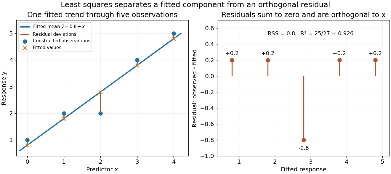
A five-point least-squares fit separates the fitted trend from residual deviations
. Details. 
The geometric reason for the fit is simple. The possible mean vectors form the column space of . Ordinary least squares chooses the orthogonal projection of the data vector onto that vector subspace, so the remaining regression residual is orthogonal to every permitted fitted direction. The least-squares normal equations express this orthogonality as . The data's explained component and unexplained component are therefore separated by the same geometry used in a Hilbert space.
The optimization definition makes sense for any observed data. Quantifying the uncertainty of the regression coefficients needs additional assumptions about the sampling and errors. With fixed of full column rank and mean-zero errors with covariance matrix , ordinary least squares is unbiased and has covariance ; the Gauss-Markov theorem compares it with other linear unbiased estimators. A normal linear model additionally makes Student t-distribution intervals and tests exact in finite samples. Model adequacy and predictive assessment remain relevant even when these calculations are available.
Two historical settings help explain the subject's appeal. Adrien-Marie Legendre's Nouvelles méthodes pour la détermination des orbites des comètes (1805) includes an appendix on the method of least squares: observations give more equations than unknowns, and squared errors provide a criterion for reconciling them. Its astronomical setting shows the motivation for combining imperfect measurements. [ref]
https://www.e-rara.ch/zut/content/titleinfo/10838079. Legendre, Nouvelles méthodes pour la détermination des orbites des comètes, 1805, appendix pp. 72–80
Francis Galton's Regression Towards Mediocrity in Hereditary Stature (1886) examines the association between parental and offspring heights and the tendency of group averages toward the population average. This is a historical use of the regression name; the modern linear model is a general statistical formulation. [ref]https://zenodo.org/records/1449548. Galton, Regression Towards Mediocrity in Hereditary Stature, 1886, original article
Cochran's theorem Created 2026-09-24 Updated 2026-09-28
Orthogonal projections of an isotropic Gaussian vector are independent. If is an orthogonal projection of rank and , then
Nonparametric regression Created 2026-09-24 Updated 2026-11-05
Nonparametric regression estimates a regression function without restricting it to a fixed finite-dimensional family.
Density estimation Created 2026-09-24 Updated 2026-11-05
density estimation constructs an estimate of an unknown probability density function from sampled observations.
Gauge transform Created 2026-09-24 Updated 2026-11-05
This local phase change is a gauge transformation of the wave function. For real and a real continuously differentiable , multiplication by is a gauge transform that preserves pointwise modulus and mass while shifting the gradient by .
NLS ground state Created 2026-09-24 Updated 2026-09-28
For the mass-critical focusing nonlinear Schrödinger equation in dimension , the NLS ground state is the positive radial solution ofIts symmetry orbit consists of the optimizers of the sharp Gagliardo-Nirenberg inequality.
Radial Sobolev inequality Created 2026-09-24 Updated 2026-09-28
Localized virial identity Created 2026-09-24 Updated 2026-11-05
For , a smooth real weight defines the localized mass . For a sufficiently regular decaying solution and a weight with the required integrability,andThese formulas follow by substituting the nonlinear Schrödinger equation and integration by parts. The Hessian controls the gradient contribution; the fourth derivative term records variation of the cutoff.
Choose , with near zero and constant outside a larger ball. The interior terms reproduce the virial identity, while the remaining terms are supported in the transition region or controlled by spatial tails. A bounded weight makes meaningful for finite mass without requiring finite variance. A blowup proof still needs estimates that control those tail errors.
Blowup alternative for the nonlinear Schrödinger equation Created 2026-09-24 Updated 2026-11-05
For the mass-critical focusing nonlinear Schrödinger equation, let be the maximal forward solution in the standard local theory. Either , orBecause Mass conservation for the nonlinear Schrödinger equation fixes , this is equivalent to divergence of .
The proof uses a local existence time bounded below for data in a bounded H1 norm ball. If a sequence had uniformly bounded H1 norms, restart the equation at with that common time interval. Uniqueness joins the restarted solution to the old one and extends it beyond , contradicting maximality.
Energy conservation for the nonlinear Schrödinger equation Created 2026-09-24 Updated 2026-11-05
For the focusing nonlinear Schrödinger equation on ,the energy functional isFor a sufficiently smooth solution with decay permitting differentiation under the integral sign and integration by parts, it is constant in time. Indeed,The cancellation is the Hamiltonian conservation mechanism: the evolution rotates the energy gradient by multiplication by . The focusing sign makes the nonlinear contribution negative, so conserved energy alone need not bound the L2 norm of the gradient.[ref]
Low-Regularity Global Solutions to Nonlinear Dispersive Equations by Terence Tao. Introduction, printed pp. 20–21: Hamiltonian evolution and formal invariants; low-regularity discussion distinguishes solution constructions
For less regular solutions the displayed computation is only formal. To inherit the identity, approximate by smooth solutions and justify convergence of both energy terms. Convergence in Sobolev space controls the nonlinear term through a suitable Sobolev embedding only in the applicable exponent range, or with additional integrability. An arbitrary weak solution must not be assumed to satisfy the identity solely because the smooth equation does.
Mass conservation for the nonlinear Schrödinger equation Created 2026-09-24 Updated 2026-11-05
For the nonlinear Schrödinger equationwith real-valued , a sufficiently regular, decaying solution with finite L2 norm conservesDifferentiating gives . Substitute . Integration by parts makes real, and is real as well, so multiplication by gives zero real part.
The real coefficient is essential to this calculation; phase covariance alone does not imply mass conservation. For an solution obtained by a well-posed approximation theory, the invariant extends from smooth solutions by continuity in the L2 norm.[ref]
Nonlinear dispersive equations: local and global analysis by Terence Tao. Section 3.4, conservation laws and their extension through well-posedness
Brzozowski automaton Created 2026-09-24 Updated 2026-09-24
Powerset construction Created 2026-09-24 Updated 2026-10-14
Extended transition of a nondeterministic finite automaton Created 2026-09-24 Updated 2026-10-03
Nonprincipal ideal in the integers adjoined a square root of minus five Created 2026-09-24 Updated 2026-11-05
In , the idealhas additive index two. If were principal, multiplication by its generator would givewhich has no solution in integers. Thus is not principal.
Dirac current Created 2026-09-24 Updated 2026-11-05
There are unlisted articles, also show them or only show them.