
Inertia tensor Created 2026-09-24 Updated 2026-10-14
The inertia tensor packages the moments of inertia about every axis through a specified point into one symmetric matrix. An axis still needs a direction: if is a unit vector, its scalar moment of inertia is . The same mass layout can therefore be easy to spin about one direction and harder about another. The inertia tensor also determines rotational kinetic energy and relates angular velocity to angular momentum in the appropriate rigid body model.
Take position vectors relative to , expressed in an orthonormal basis. For point masses , or a continuous distribution with mass density and ,Here is the Kronecker delta. Equivalently, using the identity matrix and an outer product,Every entry has SI units . The diagonal entries are axial moments of inertia; the off-diagonal entries carry a minus sign in this convention. Some texts instead define the integrals without the prefixed minus sign , , as their named off-diagonal quantities and put the minus signs into the displayed matrix. Check that convention before combining formulas. [ref] [ref]
The symmetric matrix is positive semidefinite, because its quadratic form isThe dot product and cross product identify this as a sum of squared distances when is a unit vector. A zero moment of inertia occurs precisely when all the mass lies on that axis, up to sets of zero mass. A genuine three-dimensional body with positive mass density in a volume has strictly positive axial moments of inertia. Do not confuse this inertia tensor with the mass second-moment tensor : they obey , where denotes the matrix trace.
If is fixed in an inertial frame and each velocity is , summing the individual kinetic energies and angular momenta givesThese formulas also describe angular momentum and rotational kinetic energy relative to the centre of mass of a translating rigid body. In that case the total kinetic energy in the inertial frame is . For a general moving point , the body's actual velocities include , so alone need not be its angular momentum about . [ref] [ref]
Changing the orthonormal basis changes components, rather than the physical distribution: if the columns of an orthogonal matrix are the new basis vectors expressed in the old basis, then . Changing the reference point is a different operation, governed by the tensor parallel-axis theorem. Both principal axes and principal moments of inertia must therefore be quoted with their reference point.
Structure theorem for finitely generated modules over a principal ideal domain Created 2026-09-24 Updated 2026-11-05
Every finitely generated module over a PID is a direct sum of a free module and cyclic prime-power torsion modules.
Annihilator of a module Created 2026-09-24 Updated 2026-11-05
Irreducible module Created 2026-09-24 Updated 2026-11-05
An irreducible, or simple, module is nonzero and has no submodules other than zero and itself.
Cyclic module Created 2026-09-24 Updated 2026-10-14
A module is cyclic if one element generates it: every element is for some scalar . The generating element need not give unique coefficients. The module homomorphism , , is surjective. Over a commutative ring, its kernel is the annihilator , givingThus cyclic modules are exactly the quotient modules for ideals in . For a left module over a noncommutative ring, use a left ideal and interpret the quotient as a module, with no claim that it is a quotient ring. See John A. Beachy's Abstract Algebra Online, section 10.1.
The module is generated by , and also by , whose successive multiples are . The element generates only , a submodule with three elements. A cyclic module can be infinite and free, as shows, or finite and torsion, as shows. One generator counts directions of generation, not the number of elements and not freedom from relations.
Projective module Created 2026-09-24 Updated 2026-11-05
A module is projective when every map from through the target of a surjection lifts through that surjection.
Torsion-free module Created 2026-09-24 Updated 2026-10-14
A module over an integral domain is torsion-free when with implies , equivalently when its torsion submodule is zero. Every free module over an integral domain is torsion-free, as one can check in each coefficient. Every vector space is torsion-free over its scalar field.
The converse requires hypotheses. A finitely generated module over a principal ideal domain is free if it is torsion-free, but the module over is torsion-free and not free. Any two nonzero rational numbers have a nontrivial integer relation, so a possible basis of a module could have at most one element; no single generates all rational numbers, since for . The finite-generation hypothesis cannot be dropped. See Keith Conrad's Modules over a PID, Corollary 2.6.
Free module Created 2026-09-24 Updated 2026-10-14
A free module is a module with a basis of a module : every element has exactly one expression with and only finitely many nonzero. Equivalently, the coefficient map is a module isomorphism. Existence means generation; uniqueness means linear independence in a module. For finite of size , this says , a finite free module. See Neil Strickland's Rings, Modules and Linear Algebra, section 11.
The integer lattice in the opening diagram is a free module over with basis of a module , . For example, , and comparing the two coordinates makes the coefficients unique. A different basis of a module is , , because ; in particular .
By contrast, and are linearly independent in a module, but generate only the submodule . They miss because has no integer solution. They would form a basis over the rational numbers. Even generation need not let one extract a basis of a module: the elements generate , since , but neither singleton generates it, and is a nontrivial linear relation between them. These are concrete failures of the usual vector space argument that divides by any nonzero coefficient.
The cyclic module has no basis of a module over : every element has the nontrivial relation , so no nonempty subset is linearly independent in a module, while the empty subset cannot generate this nonzero module. Specifying the scalar ring is essential: over , the same additive object is a free module with the one-element basis of a module , since each coefficient is itself a unique class in .
Quotient module Created 2026-09-24 Updated 2026-11-05
Primary decomposition theorem for finitely generated modules over a principal ideal domain Created 2026-09-24 Updated 2026-11-05
A finitely generated module over a principal ideal domain decomposes aswith finitely many irreducibles . The free rank and primary cyclic factors are unique up to associates and ordering.
Length of a module Created 2026-09-24 Updated 2026-11-05
A module has finite length when it admits a composition series of a module, and its length is the number of simple modules among the successive quotients. The Krull–Schmidt theorem concerns decompositions into indecomposable summands; the independence of composition length instead follows from the Jordan–Hölder theorem. A module without a finite composition series is assigned infinite length.
Filtration of a module Created 2026-09-24 Updated 2026-11-05
Inverse system Created 2026-09-24 Updated 2026-10-03
Short exact sequence Created 2026-09-24 Updated 2026-11-05
Determinant trick Created 2026-09-24 Updated 2026-11-05
Flat module Created 2026-09-24 Updated 2026-11-05
An -module is flat when tensoring with it preserves injections, equivalently when is an exact functor.
Tensor product of modules Created 2026-09-24 Updated 2026-11-05
For a right module and a left module , their tensor product of modules is the abelian group generated by symbols , modulo additivity in each variable andThe universal property of the tensor product of modules identifies additive maps from it with balanced maps on .
When is a commutative ring, two left modules can be used by viewing the first as a right module. The tensor product is then an -module with . For example, : the generator is killed by both and , and the universal property identifies exactly those relations. For a noncommutative ring, the left and right input actions must be specified.
Laplace integral method for a differential equation Created 2026-09-24 Updated 2026-11-05
The Laplace integral method for a differential equation seeks a solution of the formUnder sufficient convergence and regularity, differentiating in multiplies the amplitude by powers of . Multiplication by can be transferred to a derivative in by integration by parts; for example,Choosing a suitable contour and amplitude makes the boundary term vanish and turns the original differential equation into an equation for .
The amplitude equation is first order for many equations whose coefficients are linear in , as in the Laplace integral solution of a singular third-order equation. More general polynomial coefficients can produce higher amplitude derivatives, so first-order reduction is not automatic. Boundary terms, branch choices and justification of differentiating under the integral are part of the construction; merely writing a formal amplitude equation does not prove that the integral exists or solves the original problem.
Mertens function Created 2026-09-24 Updated 2026-11-05
The Mertens function is the summatory function of the Möbius function:For example, , , and . On nonnegative real inputs it is constant between consecutive integers, with . Its jump at a positive integer is , so there is no jump at a nonsquarefree integer.
The Mertens function measures cancellation between square-free integers with an even number and an odd number of distinct prime factors. The estimate says that their signed excess is negligible compared with the total length of the counting interval; through prime number asymptotic from Mertens cancellation, this cancellation implies the Prime number theorem.
Möbius inversion formula Created 2026-09-24 Updated 2026-11-05
Möbius inversion recovers an arithmetic function from its divisor sum. For arithmetic functions , the following statements are equivalent, with each equality required for every positive integer :Here ranges over positive integer divisors of and is the Möbius function. No multiplicativity assumption is needed, and both sums are finite. The right side can also be written by exchanging complementary integer divisors. [ref]
Floor and arithmetic functions by Darij Grinberg. Darij Grinberg, MIT 18.781 lecture notes, Theorem 2.5.1 and Proposition 2.5.2
The divisor sum bundles together with values at smaller integer divisors. Möbius inversion subtracts aggregates indexed by one distinct prime factor, adds those indexed by two, and continues with the alternating signs of inclusion-exclusion. A divisor containing a squared prime factor receives weight zero. The Möbius divisor-sum identity ensures that every unwanted contribution cancels exactly.
In Dirichlet convolution notation, and , where is the constant-one arithmetic function and is the Identity for Dirichlet convolution. Associativity and commutativity give the short proof:Convolving with proves the reverse implication. At , the formula reduces to because .
For a worked example, take , Euler's totient function. The totient divisor-sum identity says that , the identity arithmetic function:This identity comes from classifying the integers by their greatest common divisor with : the group with has members, since and are coprime integers. Summing the group sizes gives , as detailed under totient divisor-sum identity.
Now undo this aggregation with the Möbius function:The nonzero terms use ; vanish because they contain the square of the prime number . The four surviving integers coprime to are .
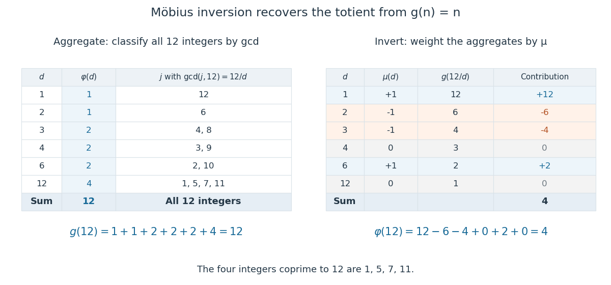
A divisor sum aggregates Euler's totient function values to 12, while Möbius inversion recovers the four integers coprime to 12
. Details. 
This example also reveals why Möbius inversion is useful: it turns an easy count of all objects into a count satisfying a coprimality restriction. Expanding over subsets of distinct prime factors givesThe product is inclusion-exclusion over multiples of the prime factors. For , it gives . More generally, whenever a counting problem produces a divisor sum, Möbius inversion lets that aggregate be reversed without solving a new system of equations.
There are unlisted articles, also show them or only show them.