
Set . Because is an orthogonal matrix, and exactly when . The preceding diagonalization givesConsequently , with equality only when . The matrix is a symmetric positive-definite matrix, not merely positive semidefinite. In the original coordinates the same identity iswhich also makes positivity transparent.
The characteristic polynomial isThus the eigenvalues are 1 and 11. Corresponding eigenvectors are and . Their dot product is zero and each has Euclidean norm . Normalizing givesThe columns are orthonormal, so . The eigenvector equations give and hence , proving the claimed orthogonal diagonalization of a real symmetric matrix.
Not unique in general. For any invertible matrix ,is another rank factorization, with the same full ranks. This is a change of basis in the intermediate -dimensional space. For example, even has different full-rank factors. Once a particular ordered basis is fixed, its coordinate matrix is unique; it is the basis choice that creates the freedom.
Choose independent columns of that form a basis of its column space, and put them in . For each column of , let be its coordinate vector in that basis; put these coordinate vectors in . The column equations give .
By construction has full column rank . The columns of corresponding to the selected basis columns are the standard vectors of , so has full row rank . This proves the requested rank factorization. When , and the corresponding empty-column and empty-row factors have the required shapes and rank zero.
False. Triviality of gives , while triviality of gives because transpose preserves matrix rank. Both conditions therefore force , contradicting the stated unequal dimensions.
True. A square matrix with matrix rank is invertible, and its transpose has the same rank. Applying the rank-nullity theorem to both and gives nullity zero in each case, so both kernels are .
False. Take , an , matrix of matrix rank one, and . Then never equals . Full column rank implies injectivity, not surjectivity onto a larger codomain.
True. The rank-nullity theorem gives . The only vector in this zero-dimensional kernel of a linear map is the zero vector.
True. Using the same transpose identity and givesThe final equality follows by multiplying and in either order and obtaining the identity. Thus the inverse is a skew-symmetric matrix as well. The invertibility hypothesis is retained throughout.
True. Transposing the inverse identities shows . If , this becomes , exactly the symmetric matrix condition. The reasoning uses the matrix inverse and transpose identities, without assuming that different matrix factors commute.
The system is consistent for every : take , since . Thus is a right inverse giving an explicit solution for every right-hand side.
All solutions are with in the kernel of a linear map represented by . The rank-nullity theorem gives kernel dimension ; the solution is unique when , and is nonunique when .
If is , then is . The equation makes every standard basis vector of a linear combination of the columns of : take the corresponding column of as coefficients. Hence the column space is all of , giving . In particular, and has full row rank.
The independent-column representation gives . Thus a vector lies in the kernel of a linear map represented by this matrix precisely when and . Writing the two free coordinates separately givesThe two displayed vectors are linearly independent, so they form a basis of the kernel. Its dimension two also agrees with the rank-nullity theorem, .
Let and . The remaining columns are and , so these two vectors span the column space. They are linearly independent: the determinant of their first two coordinates is . Therefore is a basis of the range, and the matrix rank is two.
Past exam of the waves and compressible flow course of the University of Oxford 2023 3 b ii Solution 2026-10-25
For fixed , the left side is a strictly increasing function on , with limit at and unbounded growth. The right side is a strictly decreasing function, sinceIt tends to infinity as and to one as . Their continuity and the intermediate value theorem give a crossing, and strict opposite monotonicity makes it unique. There is exactly one admissible bore speed for every .
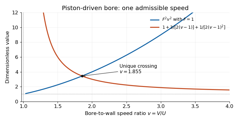
Unique intersection determining the piston-driven hydraulic-bore speed, illustrated for Froude parameter one
. Details. 
The illustrated case is ; changing moves the increasing curve without changing the existence or uniqueness argument. The vertical asymptote at expresses the growing depth ratio .
Past exam of the waves and compressible flow course of the University of Oxford 2023 3 b i Solution 2026-10-25
Let be the depth behind the bore. The wall's kinematic boundary condition makes the velocity there ; ahead of the bore the depth and velocity are and zero. Across a rightward hydraulic bore moving at , the Rankine-Hugoniot conditions areThe first gives . Substituting into the second gives , where and . Hence the piston-driven shallow-water bore obeysThe positive depth increase is consistent with the energy-loss condition in ii, now viewed in the bore's own shock frame.
Put . The squared Froude numbers follow directly from the discharge relation:Thus the jump connects supercritical flow to subcritical flow. Long surface gravity waves have speed relative to the fluid, so the characteristic speeds in the stationary frame are . Upstream both point with the flow; downstream one points against it. The jump changes whether long-wave information can propagate upstream through the local flow.
Past exam of the waves and compressible flow course of the University of Oxford 2023 3 a ii Solution 2026-10-25
Orient the flow so , and let subscripts 1 and 2 denote upstream and downstream. The mechanical energy flux is , where . Inserting the relation for in i gives the hydraulic jump head loss,An admissible jump dissipates mechanical energy, so . The denominator is positive, henceThe zero depth-change case is continuous flow. A depth-decreasing discontinuity would require an energy input at the jump; it is not the dissipative hydraulic jump selected by this model.
Past exam of the waves and compressible flow course of the University of Oxford 2023 3 a i Solution 2026-10-25
Take a unit-width control volume spanning the stationary hydraulic jump. Mass conservation makes the discharge constant. The horizontal momentum flux is , and the integrated hydrostatic pressure force on a vertical cross-section is . Momentum conservation therefore givesThese are the Rankine-Hugoniot conditions for the shallow water equations in the stationary shock frame. With depths on the two sides, eliminating the velocity gives
Past exam of the waves and compressible flow course of the University of Oxford 2023 2 c ii Solution 2026-10-25
Write the cosine in i as two complex exponentials. On a ray , the oscillatory phases are . The stationary phase method requires . By ii, the largest absolute horizontal group velocity for the occupied mode isInside this region there are stationary wavenumbers supporting appreciable wave packet contributions. Outside it no stationary wavenumber exists; oscillatory cancellation suppresses the large-time response. This explains "mainly confined": the initial Lorentzian profile already has nonzero algebraic tails, so the displayed region is not the exact support of the solution. Near its boundary the stationary points meet and the usual nondegenerate stationary-phase formula needs a transition approximation.
There are unlisted articles, also show them or only show them.