
Strong geological magnetic anomalies generally occur in rocks containing abundant strongly magnetic iron oxides, especially magnetite and titanomagnetite. Many mafic rocks, including basalt and gabbro, and some ultramafic rocks have large signatures; magnetite-rich iron formations can be exceptionally strong, while serpentinization can create additional magnetite. Actual magnetic susceptibility and remanent magnetization, rather than the rock name alone, determine the response. Sedimentary and felsic rocks are often weaker but have important exceptions.
Magnetite, titanomagnetite and maghemite exhibit strong ferrimagnetism; some pyrrhotite is also strongly magnetic. Hematite is generally much weaker in induced magnetic susceptibility, although it can carry stable remanent magnetization. Quartz and calcite have very small, usually negative, susceptibilities, and many ordinary silicates have only weak paramagnetism. A steel car exhibits strong ferromagnetism and can therefore stand out against a weakly magnetic host, but its shape and pre-existing remanent magnetization complicate the signal.[ref]
Applications manual for portable magnetometers by Geometrics. Rock-susceptibility discussion and the section “Remanent or Permanent Magnetization”.
Lay out a surveyed grid extending beyond the possible burial area into unaffected ground. Use closely spaced parallel traverses with measurements along each line; spacing should resolve a car-scale magnetic anomaly, with a finer grid over any candidate. For a shallow car, a pilot survey with roughly metre-scale spacing is a sensible starting point, refined according to anomaly width rather than treated as a universal prescription. Record position, time, sensor height, repeat readings and any nearby interference. Cross-lines and repeat stations check reproducibility. Maintain a constant sensor height on a nonmagnetic staff and remove magnetic items from the operator; map fences, gates, pipes, buildings and vehicles before interpreting an anomaly.
Operate a synchronized stationary base-station magnetometer in quiet ground while the rover surveys, or make frequent base returns if a second instrument is unavailable. A total-field magnetic anomaly is the corrected field magnitude minus a specified background:For a field-sized target, a local background estimated away from the car is often sufficient. A larger regional survey may subtract the International Geomagnetic Reference Field and an independently justified regional trend. Do not remove the car's broad anomaly by overfitting that trend.
Correct rover observations for time-varying geomagnetic field using the base record, for example . Check instrument offsets and tie-line differences, reject disturbed or poor-quality readings, and allow for differing sensor heights. Preserve localized target signals when interpolating a contour map or comparing with a magnetic dipole model. There are no compulsory gravity-style free-air or Bouguer gravity anomaly reductions for this magnetic search.
Postpone surveying during a geomagnetic storm or rapid irregular magnetic variation, when base correction may be inadequate. Avoid periods of moving farm machinery or electrical interference, and recognize that strong permanent cultural interference or highly magnetic host rock may make this particular method unsuitable. Ordinary cloud cover or darkness does not prevent a magnetic survey.[ref]
G-857 Memory-Mag operation manual by Geometrics. “Magnetic Environment” and survey/base-station operation: magnetic cleanliness, spatial gradients, and time variation.
A proton-precession magnetometer measures the scalar magnitude of the local magnetic field. Its sensor contains a proton-rich liquid, such as a hydrocarbon or suitable water-based fluid. A strong current through a coil briefly polarizes the nuclear magnetic moments, producing a small net magnetization. The polarizing field is directed sufficiently across the local magnetic field to leave a transverse component when the current is switched off.
The protons then undergo Larmor precession about the ambient magnetic field. Their rotating net magnetization induces a decaying alternating voltage in a receiving coil. Measuring the frequency determines the field:For example, gives about . The known proton gyromagnetic ratio provides an absolute frequency-to-field scale; this instrument does not measure the field's direction. Strong spatial gradients cause different parts of the liquid to precess at different rates and shorten the usable signal, which matters very close to a buried steel object.[ref]
G-857 Memory-Mag operation manual by Geometrics. Introduction, “What is a total field magnetometer?”, and “Magnetic Environment”; scalar intensity and sensitivity to gradients.
The three stable fields are:Equalities give the stable coexistence boundaries described above. In particular, a point between the two descending line extensions is not automatically a fourth field: only the lower line borders the stable corundum region on each side of the intersection. The free-energy comparisons, rather than the appearance of the complete straight-line sketch, select the stable mineral.
The stability boundary in a mineral activity diagram requires the two coexisting minerals to be stable against the third. For the forward dissolution directions of (I) and (II),A negative value favours corundum over the corresponding silicate mineral. For (III),so low silica activity favours nepheline over albite, and high silica activity favours albite. Combining these comparisons gives the stable portions:
The opposite extension of each line is metastable because the third mineral has lower thermodynamic potential there. All three minerals can coexist at the intersection in this fixed-temperature, fixed-pressure activity model.
For pure albite, pure nepheline and unit water activity, . Consequentlya vertical line through the intersection of (I) and (II). It does not depend on because the net reaction has no hydrogen or sodium ions.
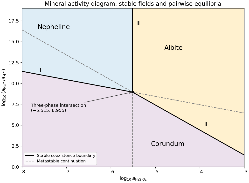

Subtract reaction (I) from reaction (II), cancelling the common aqueous ions and corundum, and divide by two. Choose the albite-to-nepheline direction:This is albite plus water converting to nepheline and dissolved silica. Standard Gibbs energies of reaction add with their stoichiometric coefficients, so logarithms of equilibrium constants do too. For this single-formula normalization,The doubled reaction has , while reversing either reaction changes the sign. Specifying the direction and normalization removes that apparent ambiguity.
Take base-ten logarithms and use dimensionless thermodynamic activities. The supplied concentration notation is interpreted in the ideal dilute-solution approximation, with a consistent reference concentration. PutWith pure solids and unit water activity, the reaction quotients are and . At chemical equilibrium, , so the two lines on the mineral activity diagram areThey have slopes and . Restricting the plotted silica activity to is compatible with their intersection,Their full straight extensions are equilibrium relations for the respective phase pairs; not every extension is a stable boundary when the third mineral is available.
The P wave source is normally the more useful depth source for the end members and for the stated approximately 50% gas case, because the predicted exceeds , making the reservoir-top arrival easier to identify, assuming comparable source and recording quality. For a horizontal reflector and vertical two-way travel time entirely through the homogeneous cap rock,or for an identified S wave arrival, with times in seconds. The reservoir's own wave speed is not the overburden wave speed used in this conversion. Nonzero-offset data require moveout correction and an appropriate overburden velocity model; no numerical depth can be obtained without a measured time.
At approximately 50% gas, Figure 1 gives , , and –. ThusThe S wave reflector is then weak because its impedance is nearly matched to the cap rock. An exact impedance match, , gives : a reservoir top can exist without producing an observable normal-incidence S wave reflection. Rounding the 50% to would suggest exactly that cancellation, but the plotted line sits slightly higher. The continuous curve crosses the cap-rock value at a somewhat greater saturation; the coarse figure does not justify a precise percentage.
There is also a smaller-saturation P wave impedance match: changes sign between zero and modest gas saturation, so it must pass through zero. Thus neither source guarantees a detectable reflector at every saturation. Joint P wave and S wave observations help distinguish a weak impedance contrast from an absent reservoir; a slower S wave speed alone is no reason to prefer it when its reflected amplitude is near zero.
Let be the fraction of the pore space occupied by gas, and let be the porosity. At fixed porosity and unchanged rock framework, the bulk density isReplacing water with much less dense gas therefore decreases the bulk density approximately linearly, as in Figure 1. The liquid and gas densities here are those at reservoir conditions.
A pore fluid has negligible static shear modulus, so the rock framework chiefly controls the effective shear modulus . If changes little, increases gently as the density falls. This does not imply that S waves travel through the pore gas itself: their restoring force comes from the connected solid framework.
The P wave speed depends on both bulk modulus and shear modulus:Gas is much more compressible than water. Even a small connected gas fraction can strongly reduce the effective fluid bulk modulus, approximately through the compliance average for a pressure-equilibrated mixture. The saturated rock's effective bulk modulus consequently falls rapidly at first, overwhelming the smaller density reduction and causing the sharp initial fall in . Once the fluid is already very compliant, further gas replacement changes the stiffness less; the continuing density decrease can then make rise again. Figure 1 assumes a particular saturation response: patchy fluids, changing effective pressure, and frequency-dependent fluid motion can alter it. The plotted is only nearly constant, so the plot should not be interpreted as an exact fixed- constitutive model.
For fugacity coefficient , use for the water activity. The solid pressure correction still uses the actual pressure . ThusLowering the water chemical potential favours the product side, which lowers the equilibrium temperature relative to part (c) under the stated constant-property model.
Adopt ideal independent mixing on crystallographic sites, with Mg and Fe sharing three positions per formula unit and the other endmember sites fixed. This gives the phlogopite and pyrope activitiesThe reaction quotient contains their ratio, since pyrope is a product and phlogopite a reactant. ConsequentlyThe site-mixing assumption is part of this numerical answer: compositions alone do not determine nonideal thermodynamic activities. More detailed activity coefficients or unequal site occupancies would need an additional model. The cube counts the three magnesium-bearing positions rather than three molecules of each mineral.
Apply the pressure correction to a mineral reaction to the solids and use the chemical fugacity of the water product. For pure solids and water vapour treated as an ideal gas,The gas contribution is already included by the logarithm and must not be counted again as an independent volume correction. With pressures in bars,
At the one-bar standard state, pure phases have unit thermodynamic activities. The Gibbs energy of reaction balance is , givingThis uses the stipulated temperature-independent reaction enthalpy and entropy differences, taken per mole of the written reaction.
There are unlisted articles, also show them or only show them.