
The population variance is , and the population standard deviation is . For a sample, the usual unbiased estimate of population variance isThe sample standard deviation measures scatter in the original concentration units; variance has squared units. Both are nonnegative, but the sample standard deviation itself is not generally an unbiased estimator of . The table's entries are interpreted as sample standard deviations for the calculations below, rather than standard errors of the mean.
The arithmetic mean is , the total measured concentration divided by the number of observations. The median is the central value of the sorted observations, or an interpolation between the two central values under the chosen even-sample convention. It is the 50th percentile.
The table's “75th quartile” means the 75th percentile, or upper quartile , with approximately three quarters of observations at or below it. Its “25th quartile” means the 25th percentile, or lower quartile . There are four quarters of a distribution, rather than 75 different quartiles. Quantile interpolation rules can differ for a finite sample; their intended population interpretation is unchanged.
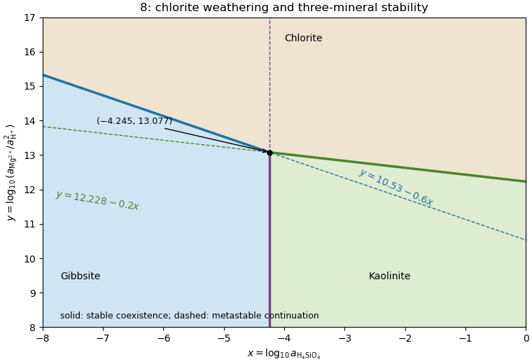
Apply upper-envelope stability for competing mineral dissolution reactions with and . For each chlorite dissolution reaction,Therefore high suppresses dissolution and stabilizes chlorite. Low favors the alteration products. To compare those products, the gibbsite-to-kaolinite reaction has : kaolinite is favored at , and gibbsite at .
The stable fields are consequently chlorite above ; gibbsite below for ; and kaolinite below for . The stable chlorite–gibbsite boundary is the left-hand part , and the stable chlorite–kaolinite boundary is the right-hand part . Their opposite extensions are metastable because the third mineral is more stable. The vertical gibbsite–kaolinite boundary is stable below and metastable above it.
The figure displays the stable upper envelope. The sign is physically testable: increasing magnesium or decreasing proton thermodynamic activity raises , inhibits chlorite dissolution, and expands the chlorite field. This direct Gibbs energy comparison avoids inferring stability merely from where three algebraic lines meet.
Subtract the chlorite–gibbsite reaction from the chlorite–kaolinite reaction. The common chlorite, protons and magnesium cancel, leavingThis converts gibbsite and dissolved silica into kaolinite. Gibbs energies of reaction add with reaction stoichiometry, so decimal logarithms of equilibrium constants also subtract:With unit water and solid thermodynamic activities, ; thus , a vertical boundary. Reversing the reaction would give and the same boundary. Its intersection with either sloping line is .
The fugacity coefficient gives . Keep the same solid thermodynamic activities and pressure correction to a mineral reaction as in part (c), changing only the water chemical fugacity:The lower water chemical fugacity makes the dehydrated assemblage more favorable, so the equilibrium temperature decreases by about . This direction is a useful independent check on the logarithm's sign.
Under ideal independent mixing on crystallographic sites, a mineral endmember's thermodynamic activity is the product of its required site fractions, one factor per mixed site. Muscovite has one K and three Al per formula unit, sanidine has one K and one Al, and corundum has two Al. Interpreting the given Al fractions as the fractions on every relevant Al/Fe site givesThus . The cubic power for muscovite includes its tetrahedral Al site and two octahedral Al sites; if site-specific fractions differed, bulk Al/(Al+Fe) alone would not determine this activity. The calculation uses the uniform-site ideal-mixing interpretation intended by the given data.
At with ideal water, solvegiving . Using the bulk mole fraction only once for a multisite mineral endmember would omit part of its ideal mixing chemical potential.
Use the pressure correction to a mineral reaction for the solids, and the gas thermodynamic activity for water. These are separate contributions: do not also add a gas-volume pressure correction after including . For this reaction,At with pure solids and an ideal gas, and the solid-activity ratio is one. ThereforeandThe pressure unit in the solid term is bar, matching the supplied . The gas logarithm is dimensionless because . High water chemical fugacity opposes dehydration and raises the equilibrium temperature substantially.
For pure phases at the reference pressure , the Gibbs energy of reaction is . Chemical equilibrium requires , soThe reaction is muscovite dehydration to sanidine, corundum and water; its positive standard entropy of reaction makes the product assemblage favored at high temperature under this constant-property approximation.
Quality is degraded by vessel and flow noise, poor receiver coupling or position uncertainty, insufficient acquisition aperture and fold, coarse sampling and aliasing, and inaccurate source timing. Finite source bandwidth limits vertical seismic resolution; shallow-water reverberations, bubble pulses, source/receiver ghosts and seismic multiples overlap primary reflections. In of water with sound speed about , the water-layer round-trip time is only about .
Seismic attenuation removes high-frequency energy, geometric spreading weakens distant returns, and heterogeneous lithology, scattering and seismic anisotropy complicate travel paths and amplitudes. Incorrect seismic velocity models misplace reflectors during seismic migration; dipping structure and out-of-plane arrivals particularly challenge two-dimensional processing. Thin layers can cause wavelet interference and tuning. Finally, even noiseless data cannot recover a normal-incidence P reflection from the stipulated zero-contrast sandstone–salt boundary: that is absent signal rather than poor recording.
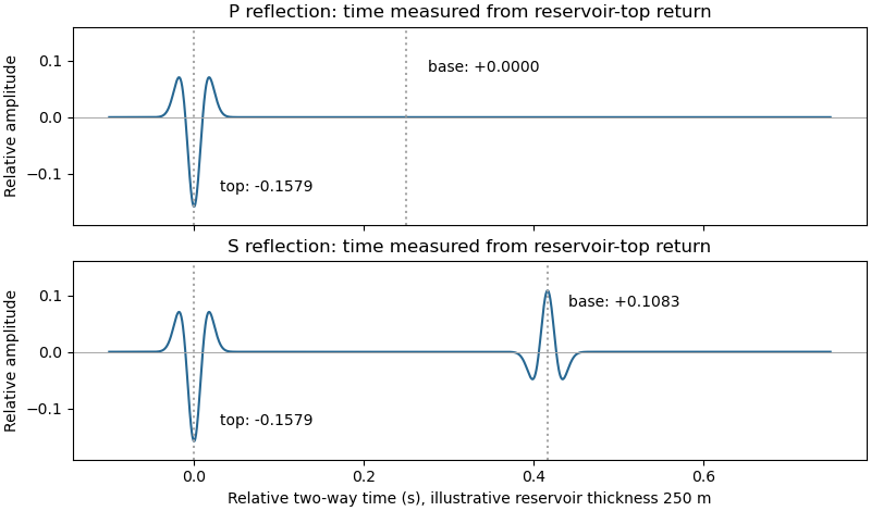
Let a positive incident stress wavelet be and measure return times relative to a receiver just above the reservoir. The top interface gives a negative P return of amplitude and no basal P return. For a separately generated and measured S wave, the top return is also negative, , while the basal return is positive, at the lower interface.
If is reservoir thickness, the basal return arrives or after the top return; no numerical is supplied. Including downward and upward transmission through the top boundary, but ignoring seismic attenuation, spreading and seismic multiples, its observed S-wave amplitude isThus the synthetic S trace has an earlier negative wavelet and a later, smaller positive wavelet; the synthetic P trace has only the earlier negative wavelet. The figure chooses solely to separate the pulses visually. Receiver electronics or a displacement convention can reverse the displayed trace polarity, so the convention must accompany the sketch.
A marine hydrophone streamer with a purely normal-incidence P source does not directly record the hypothetical S trace. A seabed multicomponent receiver and suitable S excitation or oblique-incidence seismic mode conversion are required. This distinguishes the calculated solid-layer response from what a particular acquisition system can measure.


Apply the same stress-amplitude convention to S-wave seismic impedance. At limestone–sandstone,At sandstone–salt,A stress-amplitude transmission greater than one does not violate conservation of energy: the transmitted energy fraction includes the seismic impedance ratio. For particle velocity, the corresponding pairs are and . At normal incidence in isotropic layers, pure P and pure S waves do not undergo seismic mode conversion.
Specify the amplitude convention. For incident stress/pressure amplitude one, the normal-incidence seismic reflection coefficient and stress seismic transmission coefficient areAt limestone–sandstone, and . At sandstone–salt, and . The first return reverses the chosen stress-pulse polarity; the second interface produces no normal-incidence P return.
S-wave seismic impedance is . With as documented in part (i),Unlike the P-wave case, the reservoir base has a nonzero S-wave seismic impedance contrast.
P-wave seismic impedance is . In layer order limestone, sandstone, salt,The salt's larger P-wave seismic velocity is exactly offset by its smaller printed density, so the second interface has no P-wave seismic impedance contrast in this stipulated model.
A transmitted P-wave seismic head wave occurs when its refraction angle reaches , requiring . At the limestone–sandstone boundary the ratio is : there is no P-wave seismic critical angle for incidence from limestone. A slower lower layer cannot carry that transmitted head wave.
Source notation assumption: the second printed is interpreted as . Otherwise the S-wave velocity in salt is not supplied, and this part and the salt S-wave calculations below would have no numerical answer. Retain the printed densities, including the unusually low salt value, rather than silently replacing them with typical rock properties.
With that interpretation, Snell law for elastic waves gives
There are unlisted articles, also show them or only show them.