
Global form obstruction for the Spin7 spinor 2026-10-25
The Spin group double covers SO(7). Its central kernel element acts trivially in the vector representation and as in the spinor representation. Thus a spinor Lie algebra representation does not define an ordinary SO(7) group representation. Under the same obstruction is visible because acts trivially on but negatively on .
For a spin-degenerate parabolic two-dimensional band, the Drude model gives and . Their product is the displayed mass-independent mean free path. A Fermi-surface transport interpretation requires a sufficiently degenerate electron gas; a quantum lifetime need not equal the transport relaxation time.
Small-detuning error of a Rabi pi pulse Created 2026-10-25 Updated 2026-11-05
For the Driven two-level Rabi model at fixed resonant pulse duration , put . Its transfer probability isThe sine-squared numerator differs from one only at order , while the denominator gives . Thus the leading population-transfer error is . For a target transfer error , the frequency mismatch in cycles per second should satisfy in this small-detuning regime. This is not a complete characterization of every coherent gate error.
The fugacity coefficient gives . Keep the solid pressure correction at the actual ; only the water activity uses the fugacity. ThusThe decrease from part (c) follows because lowers the chemical potential of the water product. All logarithms in these thermodynamic formulae are natural logarithms.
The compositions alone do not specify a unique thermodynamic activity model. Adopt the usual ideal, independent mixing on crystallographic sites approximation: three Mg–Fe positions per formula unit, with the other sites fixed at their stated endmember compositions. Then the mineral endmember activities areThe exponent counts the three mixing cations; treating each whole mineral formula as a single mixing site would be a different model. In particular, the magnesian biotite and garnet components here are phlogopite and pyrope.
For the written reaction, the reaction quotient iswith the other solid activities equal to one. The Gibbs energy of reaction balance therefore givesThe smaller product-endmember activity lowers the reaction chemical potential and lowers the equilibrium temperature in this model. Nonideal activity coefficients or unequal occupancies of crystallographic sites would require further information rather than a revised universal numerical answer.[ref]
Use the pressure correction to a mineral reaction for the solids, with . The water contribution must instead use its chemical fugacity. For pure solid phases and water vapour treated as an ideal gas, , givingThe last term already accounts for the gas-pressure contribution; adding another gas-volume correction would double count it. The pressure ratio inside the logarithm is dimensionless.
At the one-bar standard state, pure mineral endmembers and water vapour treated as an ideal gas all have unit thermodynamic activity. The Gibbs energy of reaction is . Setting it to zero givesThe quantities are taken per mole of the reaction as written. The simplified result uses the stipulated temperature-independent enthalpy and entropy differences.
At , the displacement expansion is . Fourier orthogonality givesDifferentiating the modal solution at zero gives , soThe factor is required because the derivative of at zero is . The dimensions agree: and are displacements, while the sine coefficients of are velocities. These projections also establish uniqueness within the finite-energy solution class.
The wave equation and its homogeneous Dirichlet boundary conditions are linear, so any finite linear combination of the separated normal modes is another solution. More strongly, the Fourier sine basis is complete in L2 space on . Expanding the initial fields in this basis yieldsCompleteness of the Fourier sine basis is the reason the expansion covers general data; linearity alone would not prove that every solution has this form. The convergence and differentiation are understood in a function space appropriate to the data. For finite wave energy, one can take and , obtaining an energy solution; stronger smoothness and endpoint compatibility give a classical solution.
For each spatial normal mode, the temporal equation is , with angular frequency . HenceThe ordinary frequency is ; it should not be confused with the angular frequency used in the sine and cosine arguments.
For , the harmonic oscillator equation gives . The condition at zero requires , and the condition at requires . A nonzero normal mode therefore hasA multiplicative normalization has been absorbed into the temporal amplitude. The candidate is affine and the two zero endpoint values force it to vanish. A positive separation constant gives hyperbolic functions, whose two zero endpoint values likewise give only the trivial solution. Negative adds no new eigenfunctions because it only reverses their signs.
Use separation of variables with a nontrivial product . Substitution into the wave equation on a string gives . Wherever the factors are nonzero,The left side depends only on and the right only on , so both are a constant. For nontrivial fixed-end solutions this constant is negative: multiplying by and integrating, using the homogeneous Dirichlet boundary conditions, givesWrite it as . The separated equations are thereforeThese equations extend across the zeros of and ; the division is a derivation device, not a restriction excluding their nodes.
The wave equation is second order in time. Even one normal mode obeys a second-order ordinary differential equation, so its initial displacement and initial velocity are independent data. Physically they specify stored elastic deformation and the initial motion.
The heat equation is first order in time; its initial temperature already fixes the instantaneous time derivative through the spatial Laplacian. It needs one initial field. In either case spatial boundary conditions remain necessary and are not substitutes for initial data. Classical fixed-end string data must satisfy the appropriate endpoint compatibility, including and, when endpoint velocities exist, .
Since tension is a force and is a linear mass density,Thus has units . It is the transverse wave speed of the ideal uniform string. The wave equation on a string assumes small transverse slopes, constant positive tension, positive uniform linear mass density, and negligible damping and bending stiffness.
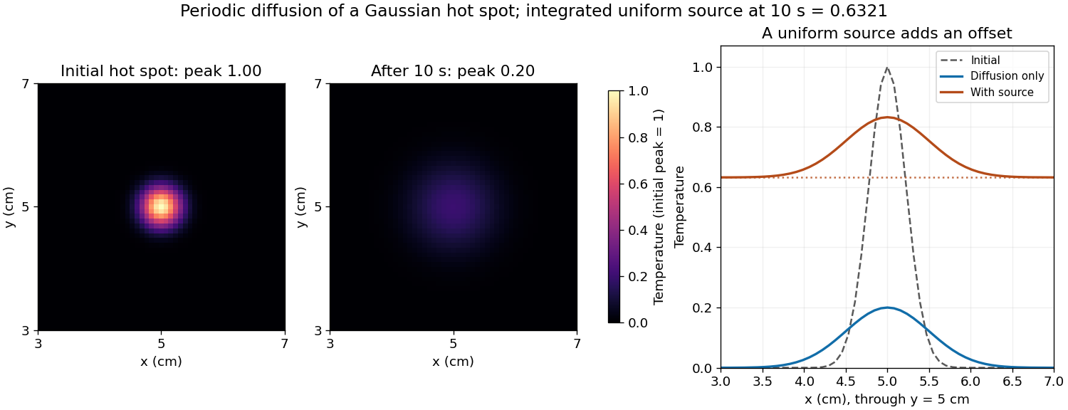
The uniform source adds a background without changing the spatial gradients relative to the unforced solution:At the offset is . On the corrected grid the central peak is therefore about , and regions far from the hot spot are near . The hot spot's broadening is unchanged; the source is spatially uniform. The spatial mean of a periodic heat equation rises by the same amount, tending to a total increment of one temperature unit as .
A spatially uniform source changes only the zero Fourier mode. Its exact integrated increment over a time step beginning at isThe unnormalised two-dimensional discrete Fourier transform stores a constant field as in element This replacement uses the original variable names and MATLAB indexing. The uniform forcing of a periodic heat equation is integrated exactly in time here. No source multiplier is applied to the other modes, and the zero-mode homogeneous multiplier equals one. Adding only
(1,1).[ref]fft2 documentation by MathWorks. The forward defining sum has no normalization; the linked inverse definition includes the factor .
Keep the existing homogeneous exponential multiplication and add this source increment to that element:for i = 1:nt
t = (i-1)*dt;
u_hat = u_hat .* exp(-alpha*K2*dt);
dq = exp(-t/10) - exp(-(t+dt)/10);
u_hat(1,1) = u_hat(1,1) + nx*ny*dq;
enddq to the unnormalised coefficient would underestimate the physical temperature increment by the factor .Aliasing occurs because a sampled grid cannot distinguish certain different continuous Fourier modes. With spacing , modes and agree at every sample point. Frequencies above the Nyquist frequency can therefore be misidentified as lower frequencies, changing the resolved spectrum and its subsequent diffusion rate.
For the corrected grid, and the maximum resolved angular wavenumber is approximately . The initial Gaussian function has spectral envelope proportional to . At that one-coordinate cutoff the factor is about , so the omitted high-frequency tail is tiny. Its continuation mismatch at the distant edges is also tiny. Significant aliasing is not expected for this resolved, smooth initial condition.
The linear constant-coefficient heat equation only damps existing modes; it does not generate higher frequencies through nonlinear products. An unresolved narrow peak, a sharp edge or a nonlinear source would require a separate resolution assessment. The duplicated-endpoint grid issue described above should not be diagnosed as high-frequency folding.
Diffusion smooths and broadens the hot spot while conserving its integral. For an isolated two-dimensional initial profile , the Gaussian hot spot under diffusion isHere and , giving a width parameter of and a peak of in the initial temperature units. The periodic-grid calculation agrees to displayed precision because the periodic copies are far away. Running the endpoint-inclusive listing as written instead gives a sampled initial peak near and final peak near ; the difference is consistent with the coordinate-grid issue, rather than a different diffusion law.
Increasing positive thermal diffusivity at fixed time produces a wider, lower peak. Each nonconstant Fourier mode decays faster, while the spatial mean of a periodic heat equation remains fixed. The profiles approach a uniform mean at long times under these periodic boundary conditions.

- Lines 1–7 set the grid dimensions, domain lengths, thermal diffusivity and time interval. The elapsed time is .
- Lines 9–10 supply coordinates, subject to the periodic-grid correction above. Lines 16–17 sample the initial Gaussian function.
- Lines 11–14 construct the discrete Fourier transform frequency order and . Negative frequencies occupy the second half of each array. This is the discrete version of replacing each spatial derivative by multiplication by .
- Line 20 computes the two-dimensional Fast Fourier transform. Lines 22–24 multiply every mode by at every step, implementing the modal solution derived above.
- Line 26 performs the inverse discrete Fourier transform. Taking the real part removes tiny imaginary roundoff errors; conjugate symmetry of the exact transformed real data already guarantees a real result.
- Lines 28–42 display the initial and final arrays. A common colour scale is needed to compare their peak temperatures; independent automatic colour scales can hide the decrease in amplitude.
For this linear homogeneous problem, the exponential update is exact for the retained modes, apart from roundoff error. It is not a forward Euler method step and does not require the explicit finite-difference diffusion stability restriction. Sampling, periodic modelling and spatial resolution still matter.
- Constant thermal diffusivity makes the Fourier spectral method diagonal: each Fourier mode can be evolved by its exact exponential multiplier.
- The smooth initial Gaussian function has rapidly decaying Fourier coefficients, so a moderate grid resolves it well. The Fast Fourier transform provides an efficient change between the spatial grid and those coefficients.
- A discrete Fourier transform describes a periodically repeated array. Opposite edges are identified by periodic boundary conditions; this is a periodically continued plate model, rather than a plate with prescribed cold or insulated edges.
- The initial hot spot is far from those edges. Over the stated short interval its width remains much smaller than the side length, so the periodic images have negligible influence near the centre. At sufficiently long times, periodic diffusion tends to the conserved spatial mean.
For consistency with the supplied wavenumbers, use an FFT grid on a periodic interval: , , and similarly for . In MATLAB, replace the endpoint-inclusive coordinate definitions by
x = (0:nx-1)*Lx/nx; and y = (0:ny-1)*Ly/ny;. The supplied linspace arrays instead have spacing while the Fourier multipliers assume . Including both copies of the periodic endpoint creates a grid inconsistency, separate from high-frequency aliasing. There are unlisted articles, also show them or only show them.