
In pure QCD, different incoming and outgoing quark flavours allow only the tree-level -channel gluon graph. A quark-gluon vertex preserves flavour, so no flavour-changing -channel exchange is available. Label the incoming momenta and outgoing momenta . For transparent spin traces, use the auxiliary metric and its usual gamma matrices; the positive-energy Mandelstam variables areThis is a consistent change of metric notation, not a change of the physical invariants. Define the fixed-index colour tensor . Up to an irrelevant common phase,The indices label incoming colours and outgoing colours. Averaging over the two spins of each incoming particle and summing the outgoing spins givesThe gamma-matrix trace identity makes the contractionFor instance and the crossed products are . Therefore, before the remaining colour sum and average,Here the bar averages spins only; it does not silently include the colour average requested next.
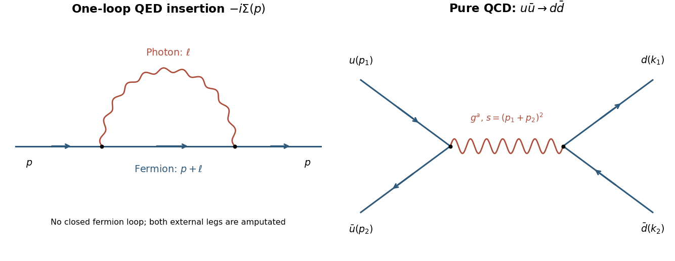

Multiply the supplied Feynman gauge propagators before reducing the numerator. Their two factors and the source's Clifford algebra implyFor example, contracting the numerator before the propagator factors gives ; the extra minus from reverses both signs.
Use a Feynman parameter on the massive denominator and shift . The combined denominator isThe term odd in integrates to zero in dimensional regularization. The pole can be evaluated away from on-shell infrared singularities; its local ultraviolet coefficient is independent of . With the source's master integral,Terms proportional to multiply the pole into a finite term, so they do not change this result. The counterterm kernel from 1ai is . Cancelling therefore givesThe distinction between mass definitions matters. Since ,Equivalently the mass-dependent part of the counterterm density is , because its definition includes the explicit minus sign in . In the alternative convention , replace every here by . These are ultraviolet minimal-subtraction poles, not the finite on-shell mass correction. The Ward identity also fixes ; the photon coefficient requires its own two-point function and is not obtained from this graph.
At second order in the interaction term, attach the two external fermion fields to different vertices and contract the remaining two fermion fields with each other and the two vector fields with each other. The factor in the expansion is cancelled by the two ways to assign the external ends. There is no closed fermion loop, and hence no extra closed-loop fermionic sign.
After removing the two external Dirac propagators, the internal momentum assignment for the photon and for the fermion gives the one-loop insertionThus the insertion is proportional to exactly the propagator product specified in the source. Define . With Fourier convention , the reduced free inverse kernel is , since the printed Dirac propagator equals . Repeated insertions giveThe factors of and the sign of the named self-energy are convention dependent; the cancelling counterterm is fixed once this insertion convention is specified. The internal photon joins two vertices on one directed fermion line, as in the first panel of the figure in 1b.
Choose the covariant derivative , so the interaction term is . The gauge transformation is and . The derivative of this local phase cancels the added vector-potential term in , making gauge-invariant.
For renormalized fields and parameters, a complete local QED counterterm parametrization isWith , , the definitions are , , and . In particular is the coefficient in the Lagrangian density, not just .
The Ward identity requires in a gauge-preserving renormalization scheme. The kinetic and vertex counterterms then combine into , so gauge invariance is explicit and . A photon mass term is not an allowed counterterm in unbroken QED. For perturbative inversion one separately adds gauge fixing, , taking in Feynman gauge. That quantization term is not itself part of the gauge-invariant density. The Abelian Faddeev-Popov determinant is field independent for this linear gauge and introduces no interacting ghost contribution.
For any fixed , the source contribution obeys , because and . Equality occurs only at when . Thus the global ground state lies on the positive first axis. Minimize there:For , . For , , so increases strictly from to . There is exactly one root , and it is the unique global minimum. ThereforeThis argument selects the true ground state even if the full cubic has additional negative stationary roots.
Expand , , . The source is linear, so it shifts the expansion point but has zero Hessian matrix. The scalar mass matrix is diagonal at the new vacuum expectation value:Eliminating with the stationary equation givesAll three squared masses are positive. The masses themselves are the positive square roots of these expressions.
The source explicitly reduces the stated SO(3) symmetry to SO(2); the selected vacuum state preserves that remaining SO(2). There is consequently no spontaneously broken exact continuous global symmetry in field theory to which the Goldstone theorem applies. For small , the two angular excitations are pseudo-Goldstone bosons. Their squared masses vanish as , while and .
Put . Completing the square in the scalar potential givesSince , its global minima form the vacuum manifoldHere denotes the positive square root of the parameter . The origin is a local maximum, not a ground state. Choose . Its stabilizer subgroup is the SO(2) subgroup of rotations in the plane, so the stated SO(3) global symmetry in field theory is spontaneously broken to SO(2).
Write , , . The kinetic terms stay canonically normalized, while the scalar mass matrix isEquivalently, the quadratic scalar potential is . Therefore the particle masses areThe two angular Goldstone bosons match . The radial displacement changes and costs potential energy, giving the massive Higgs mode. These are tree-level masses; the Goldstone theorem protects the angular zero-mass modes in the exact global theory.
The Goldstone theorem states that spontaneous breaking of a continuous internal global symmetry in field theory in a local relativistic quantum field theory produces a zero-mass Goldstone boson for each independent broken generator, under the usual positive-state-space and conserved-current hypotheses. For there are symmetry-required Goldstone bosons. This count assumes a Lorentz-invariant vacuum state; nonrelativistic counting can differ.
At the classical level, invariance of the scalar potential gives . Differentiating at a stationary vacuum expectation value yieldsThese are the Goldstone directions in the scalar mass matrix. Broken generators have , so their independent directions have zero quadratic mass with a canonical kinetic term. The theorem guarantees these modes; it does not exclude further accidental zero-mass modes. A local gauge symmetry is a redundancy and does not meet the physical global-symmetry hypothesis: the Higgs mechanism can instead supply longitudinal particle polarizations of massive gauge bosons.
Both -channel annihilation and -channel gluon exchange are now allowed. Their spin sum factors are the Bhabha scattering factors with . Their color charge tensors, with the external indices of Solution, areEach squared term has . The cross term instead has the color averageTo evaluate it, use the SU(N) fundamental completeness relationThis follows by completing the orthogonal basis of traceless Hermitian matrices with the identity. Since , it gives , and henceMultiplying the two squared Bhabha scattering terms by and its cross term by givesFor the SU(3) gauge group, this isThe negative color charge overlap reverses the sign of the QED interference. Since , this cross contribution is positive in the physical region. No additional spinor calculation is needed; all the new information is in the SU(N) fundamental completeness relation.
The two Bhabha scattering tree-level Feynman diagrams are the two panels of Solution with a photon mediator: -channel annihilation with internal momentum , and -channel exchange with internal momentum . Each interaction vertex preserves the electron species. There is no independent -channel Feynman diagram, since the outgoing electron and Positron are distinguishable.
Removing the color charge factor from Solution and replacing by givesCrossing symmetry interchanges and for the exchange Feynman diagram, givingSquaring the sum of the two scattering amplitudes also produces the interference term . The given third term must be this cross term: it has both propagator denominators , whereas a squared individual Feynman diagram has or . With the correct relative fermionic sign, its value is . ThusThe coefficient of the last displayed fraction is positive, but and in the physical scattering region, so this interference is destructive. The relative sign originates in the two possible external fermion contractions; changing an external-state phase changes both scattering amplitudes together.[ref]
Quantum Field Theory by David Tong. §6.6, Electron Positron Scattering: annihilation and exchange spinor contractions and their relative sign
There is one tree-level Feynman diagram: annihilation of the up quark and its antiquark into an -channel gluon, followed by production of the down quark and its antiquark. A gluon interaction vertex preserves quark flavor, so a -channel line joining the incoming up quark to the outgoing down quark is impossible.
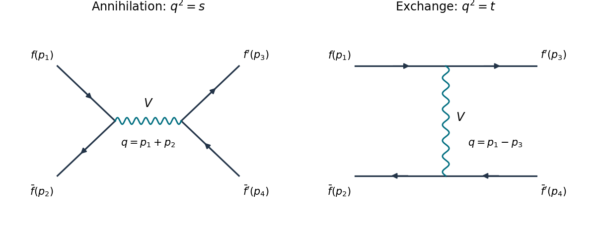
Annihilation and exchange channels with labelled external momenta
. Original Feynman diagrams, with arrows denoting fermion flow. The left panel with and is the distinct-quark flavor process. Both panels with describe Bhabha scattering; both with and describe identical-quark flavor scattering. The wavy internal line stands for the indicated vector mediator. Details.
Let label the initial quark, initial antiquark, final quark, final antiquark color charges. Up to an irrelevant common sign, the scattering amplitude isThe Mandelstam variables are , , , with in the zero-mass limit. The spin sum uses , and the initial spin average contributes . The resulting two gamma matrix traces contract toThe initial color average contributes . Summing final color charges gives the distinct-flavor quark scattering color factorThereforeEquivalently for the QCD coupling . There is no initial gluon spin average: the gluon is internal.
Past exam of the advanced fluid dynamics course of the University of Oxford 2016 2 c ii Solution 2026-10-25
The component of the stationary constitutive equation isInsert and . The coefficient of becomes , givingFor , the small-rate shear stress is . At large positive rate, and the shear viscosity decreases as . The shear stress is odd in rate, reaches a positive maximum atand decreases thereafter. The original plot displays this homogeneous constitutive curve. Its decreasing branch can permit shear banding; the local model alone supplies neither an interface-selection rule nor a guaranteed stable homogeneous realization.
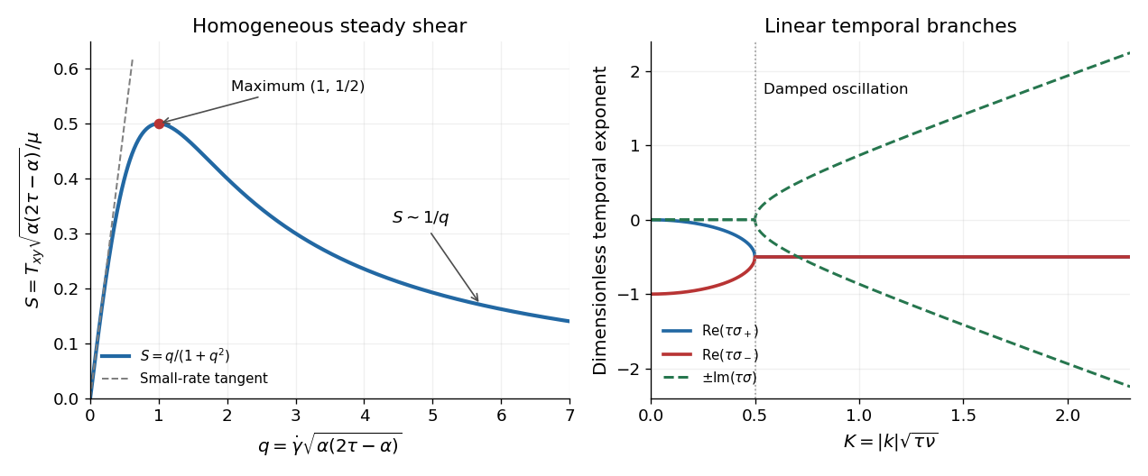
Homogeneous shear stress and the two temporal branches of the linear response
. The steady curve uses q equal to the shear rate times the square root of alpha times (2 tau minus alpha). The spectral panel uses K equal to the wavenumber magnitude times the square root of tau times nu. These are distinct nondimensional variables. Details.
This is a Johnson-Segalman fluid without an added Newtonian fluid solvent contribution. To identify conventions explicitly, set and , with the spin tensor. The derivative appearing in the constitutive equation becomesthe Gordon--Schowalter derivative. Its usual slip interval corresponds to , while a nonsingular genuinely shear thinning curve requiresAt the model is the Upper-convected Maxwell model; at it is the lower-convected derivative counterpart, and both have constant shear viscosity in this test. At the derivative is the Jaumann derivative, giving the corotational Maxwell fluid. Merely requiring is insufficient: for the denominator is , which vanishes at and then gives a negative steady shear viscosity. There is no solvent-induced large-rate plateau in the stated equation.
Past exam of the advanced fluid dynamics course of the University of Oxford 2016 2 c i Solution 2026-10-25
Let and use for the source's velocity gradient convention. Seek the homogeneous stationary stress reached under steady simple shear flow. The material derivative of that stress tensor vanishes. In the plane,The , and components of the constitutive equation give, respectively,Thus, putting and using the shear stress calculated below,The out-of-plane shear components vanish on the homogeneous branch. The two normal-stress differences areThe ratio is defined at nonzero shear when ; at both differences vanish, and the displayed constant is their limiting ratio. An arbitrary isotropic pressure in the total Cauchy stress tensor cancels from both differences; it is not an arbitrary addition to the constitutively defined extra stress itself.
Past exam of the advanced fluid dynamics course of the University of Oxford 2016 2 b iii Solution 2026-10-25
Eliminating the shear stress from the two linear equations gives the Maxwell shear-wave dispersion equation in physical space,where is the kinematic viscosity. Substitution of a Fourier mode givesThese are temporal exponents: the oscillation angular frequency is the imaginary part of , with the sign determined by the selected time convention. For both exponents are real and nonpositive. At equality the repeated exponent is ; generic solutions include . Above the threshold the modes are damped propagating shear disturbances:At large their phase velocity tends to .
For the limit at fixed and , expansion of the square root givesAfter a short initial relaxation, the surviving branch obeys the diffusion equation of a Newtonian fluid. The fast branch disappears on the vanishing viscoelastic relaxation time; at the two exponents are exactly and . This limit is not uniform in : modes with of order still sample the oscillatory transition. If instead is held fixed as , then and the fixed- slow exponent tends to zero. The ordinary Newtonian fluid limit therefore specifies which material parameter is held fixed.
Past exam of the advanced fluid dynamics course of the University of Oxford 2016 2 b ii Solution 2026-10-25
Linearize about a relaxed state with constant mass density . In the unforced momentum conservation equation , the component of the pressure gradient is zero for a freely evolving unidirectional flow independent of . A prescribed external pressure gradient would add a forcing term.
For , incompressibility is automatic and the only nonzero entries of the rate-of-strain tensor are . Products of stress and velocity gradient are quadratic in the small amplitude. The constitutive equation consequently becomes to first order. With , its shear component and the component of momentum conservation areThe diagonal stress components have only homogeneous relaxation at this order and vanish if initially relaxed. In particular, does not enter this linear response.
Past exam of the advanced fluid dynamics course of the University of Oxford 2016 2 b i Solution 2026-10-25
When deformation is stopped, the rate-of-strain tensor and velocity gradient vanish, leaving . HenceThe positive constant is the viscoelastic relaxation time. For slow weak deformation, all the transport and quadratic terms are smaller than , so . Thus is the zero-rate dynamic viscosity, measured in stress times time. The corresponding short-time shear modulus of the Maxwell fluid response is . The source's has units of time, since must have units of stress.
Adjoint branching from G2 to long-root A2 2026-10-25
The Adjoint representation of G2 has one weight at each of its twelve roots and two at zero. Its six long roots form the A2 root system; together with the two zero weights they give the Adjoint representation of SU(3). The remaining six short roots form the weight systems of its defining representation and dual representation. Hence restriction to the long-root SU(3) gives . This is a branching of a representation; the complement is invariant under the subgroup, not under the full G2 action.
Weight system 2026-10-25
The weight system of a finite-dimensional Lie algebra representation is its collection of weights with their weight multiplicities. Restriction to a Lie subalgebra projects each weight to the smaller Cartan subalgebra, retaining and combining weight multiplicities. Grouping the resulting weights into irreducible weight systems computes the branching rule.
Suppose two dissolution reactions to a reference mineral have been normalized to the same amount of a conserved reference component. After division by the same positive energy factor, let their Gibbs energies of reaction be and . Their relative thermodynamic potentials can then be written as displayed. The stable mineral has the smallest potential.
It follows that is stable below , mineral 1 is stable where and , and mineral 2 is stable where and . The two nonreference minerals coexist stably where . Their equality below that height is a metastable continuation. This comparison proves the stable lower envelope and selects which portions of the pairwise mass-action lines belong on the mineral activity diagram.
Spinor tensor square for so5 2026-10-25
For the B2 root system with long simple root first, the four-dimensional spinor representation has highest weight . Its symmetric square has highest weight and dimension ten, so it is the Adjoint representation. The exterior square has the four nonzero defining weights and two zero weights; it splits into the five-dimensional vector representation of highest weight and a trivial representation. Thus the tensor square decomposes as displayed. The invariant alternating bilinear form reflects the pseudoreal representation structure. The spinor representation is a group representation of the Spin group , while its tensor square descends to .
Choose five Hermitian four-by-four matrices obeying the Euclidean Clifford algebra relations . For , the displayed anti-Hermitian matrices satisfy the Special orthogonal Lie algebra Lie bracket relations. A direct proof first establishes , then applies the commutator product rule to . One explicit choice is , , , , , with the Pauli matrices. The Cartan subalgebra operators and have simultaneous eigenvalues , identifying the four-dimensional spinor representation. A full rotation acts as , proving it does not descend to .
There are unlisted articles, also show them or only show them.