
Write for each component's thermal penetration depth. Its contribution at depth isThus its amplitude is multiplied by and its wave phase lags the surface by radians. The corresponding unwrapped time lag is ; a phase measured from a single periodic signal is observable only modulo .
Higher-frequency variations have smaller penetration depths. In particular,The daily oscillation is therefore strongly attenuated at depths where a substantial annual oscillation survives. This is a thermal diffusion wave, whose phase lag is not the arrival time of a sharp thermal front. The displayed solution is the established periodic response; an additional transient would depend on initial subsurface data not needed for this interpretation.
Apply a Fourier transform or discrete Fourier transform, retain the desired low-frequency coefficients and attenuate those in the high-frequency noise band with a low-pass filter, then invert. For a real signal, apply matching gains at positive and negative frequencies to preserve Hermitian symmetry.
Parseval identity for Fourier series shows what an ideal coefficient cutoff does: the output mean-square signal power is the sum of the retained squared coefficients, and cannot exceed that of the unfiltered input. Much of the high-frequency noise can be removed, but a finite cutoff also removes genuine square wave harmonics. Its edges become less sharp, and a sharp spectral cutoff can exhibit the Gibbs phenomenon. There is no claim of exact recovery if the noise overlaps the retained band. Noise already folded into low frequencies by aliasing cannot in general be removed merely by discarding the high-frequency bins afterward.
Most of the mean-square signal power lies at low frequencies. Each nonzero coefficient has magnitude , so its power contribution decreases as . The pair at the fundamental frequencies alone containsof the total. The first three positive odd harmonics, together with their negative-frequency partners, contain about . The harmonic power of a square wave still has a nonzero tail: higher harmonics are needed to reproduce sharp edges even though their combined power is small.
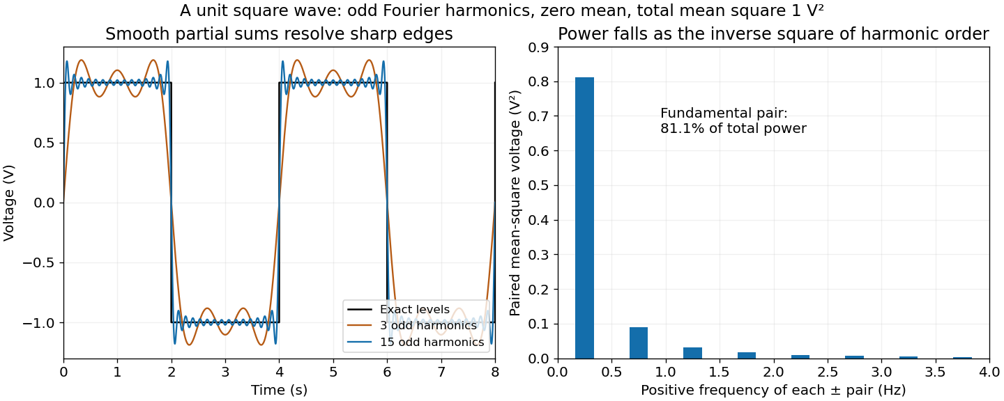

Use Parseval identity for Fourier series with the coefficient normalization above. Only odd nonzero indices contribute; summing the positive and negative indices givesThusThe factor of two from the negative frequencies is essential. The discontinuities do not obstruct Parseval's identity, which is a statement about L2 space.
The squared signal equals except at irrelevant isolated jump times. Its mean-square signal power is thereforeHere “power” has the signal-processing definition specified in the question. To convert this voltage mean square into electrical power in watts, a load electrical resistance would also be required: .
The zero Fourier coefficient is . For a nonzero integer , integrate the two constant halves:ConsequentlyThe complex Fourier series is . The negative-index coefficients are the complex conjugates of the positive-index ones, as required for a real signal. Combining each pair gives the equivalent real expansionAt a jump, pointwise convergence of a piecewise smooth Fourier series gives zero, the average of the two one-sided limits. The value assigned to at isolated jumps does not affect its Fourier coefficients or mean-square signal power.
Multiply the complex Fourier series by and integrate over one period. Fourier orthogonality removes every term except the one with index , givingFor general square-integrable functions, this is an orthogonal projection onto the corresponding Fourier mode. It remains valid when the expansion converges only in L2 space: integrate finite Fourier partial sums first, then pass to the limit using the Cauchy-Schwarz inequality. No unjustified pointwise exchange of an infinite series and an integral is needed.
Choose a fixed time increment , let , and approximate by . The Backward Euler method evaluates the transport term at the new time:Rearrange to the linear systemAlthough is a singular matrix, is an invertible matrix for every . In each row, its diagonal entry is and the sum of the absolute values of its off-diagonal entries is ; hence it is a strictly diagonally dominant matrix. Its Gershgorin discs have centre and radius , excluding zero. In particular, the zero eigenvalue of becomes an eigenvalue of .
- Form once. Compute a Pivoted LU decomposition , storing the permutation matrix , the unit lower triangular matrix , and the upper triangular matrix .
- Set .
- At each step form . Solve by forward substitution, then solve by back substitution.
- Advance and repeat until the desired final time. Choose the fixed increment so the final time is an integer multiple of , or refactor if a shorter final step is used.
Both triangular solves use the factors of . The LU factorization of the singular transport matrix from part (a) is not a solver for this new linear system. No matrix inverse needs to be formed. Since and are fixed, the same LU factorization serves every step; only the right-hand side changes. A varying would give without changing these factors.
As a check, multiplying the update by givesexactly reproducing the inventory balance at the sampled times, apart from roundoff error. The Backward Euler method has temporal global error for smooth solutions, so its A-stability does not remove the need to select for accuracy.
There are unlisted articles, also show them or only show them.