
A reverse or thrust fault earthquake is the expected end member: a hanging wall moves upwards relative to its footwall, accommodating north–south tectonic shortening. A plausible double-couple seismic source focal mechanism has an approximately east–west fault strike, a moderately north- or south-dipping fault plane, and up-dip fault slip. For example, right-hand-rule strike , southward fault dip about , and fault rake specify a pure thrust mechanism.
In a lower-hemisphere equal-area plot, with shaded regions denoting compressional P first motions, this focal mechanism has a shaded central region and two unshaded outer lobes. The P axis is approximately horizontal north–south and the T axis approximately vertical for a symmetric idealization; for a single plane their axes are slightly tilted. The P and T axes of a double-couple seismic source need not exactly equal the regional principal stress axes. The nodal curves represent both the fault plane and its auxiliary plane; additional evidence is needed to choose between them.[ref]
Focal mechanisms or beachballs by United States Geological Survey. Lower-hemisphere compression shading and the ambiguity between the two nodal planes.
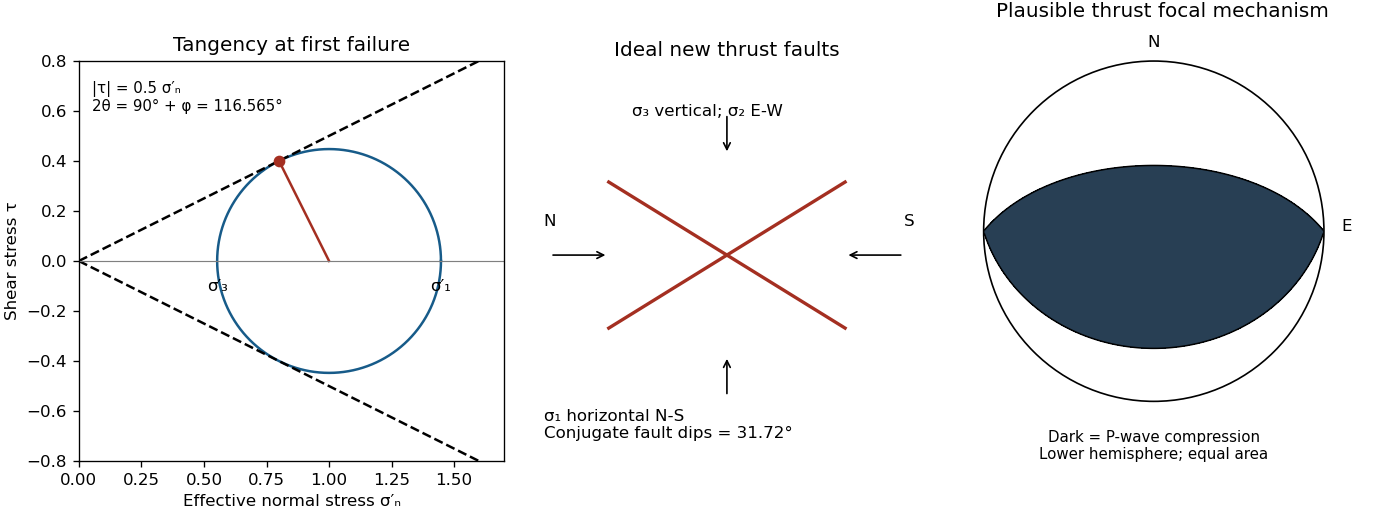

Use compression-positive principal stresses, . For the intended thrust fault regime during approximately north–south tectonic shortening, the likely orientations areA locally horizontal traction-free surface motivates taking one principal direction as vertical, while the strong north–south compression selects the maximum horizontal principal stress. The expected fault strike is then approximately east–west.
This ordering assumes the two horizontal compressions exceed the vertical principal stress. North–south shortening by itself does not establish the magnitudes of all three: if the vertical principal stress were intermediate, strike-slip faulting would instead be possible. The answer above is the simple compressional end member used in the following parts.
Assume that the intrusion has a positive magnetic susceptibility contrast, that induced magnetization dominates its remanent magnetization, and that the local present-day geomagnetic field points roughly northward and downward, as in this northern mid-latitude setting. Writewhere is the anomalous magnetic field and the last expression assumes . A total-field magnetic anomaly measures a field projection, so it need not have the same sign everywhere above a high-susceptibility body.[ref]
The 100 km east–west extent makes an approximately two-dimensional, east–west-striking body a useful model away from its ends. On a profile drawn north on the left, south on the right, the expected normally induced response has a subsidiary negative lobe on the northern side and a stronger positive lobe over the body, displaced towards the south. The northward horizontal field component makes the anomaly asymmetric; its downward component produces the dominant positive response. The field falls back towards the regional value away from the intrusion. Broad bodies can have edge shoulders or a broad central high, so the sketch represents a qualitative shape rather than one uniquely specified curve.
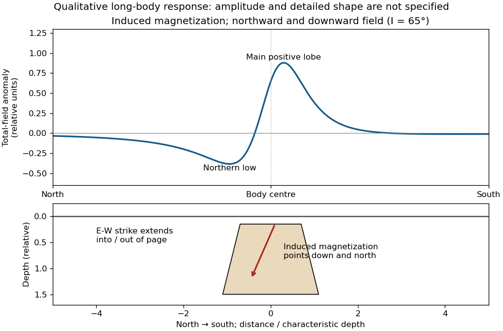

An exactly vertical inducing field would remove this north–south skew for a symmetric induced body. Real magnetic inclination and magnetic declination should be taken from a suitable geomagnetic field model for the survey date and location; no exact local value is supplied here. Strong oblique or reversed remanent magnetization can shift or reverse the lobes, and heterogeneous magnetic susceptibility, body dip and three-dimensional end effects can alter the profile. Higher magnetic susceptibility alone does not determine a unique amplitude or polarity pattern without these qualifications.
For the two negative gravity anomalies in the actual Figure 1, examine where the steepest flanks occur within the total fall into the trough. The solid upper intrusion profile has maximum slope relatively low on its flanks, close to the flat trough; its body widens downwards. The lower basin profile has maximum slope relatively high on its flanks, near the shoulders; its body narrows downwards. The dashed gradient traces and arrows mark these transitions. The signed derivative changes sign on opposite sides of a symmetric trough; a plot of gradient magnitude instead gives two positive peaks.
A shallow edge controls a relatively abrupt local change, whereas deeper geophysical density contrast spreads its effect over greater horizontal distance. Downward-narrowing geometry leaves relatively more of the anomaly associated with the shallow broad part, placing the strong flank change nearer the outer shoulders. Downward-widening geometry adds a broader deep contribution beneath the narrow outcrop, shifting the inflection towards the lower part of the trough. Thus the location of a flank's maximum slope relative to its shoulder and minimum is more useful here than the shared peak alone.
A symmetric constant-density body with vertical sides gives a symmetric negative trough with paired rounded flanks; for a broad shallow body the main slope changes occur approximately halfway down those flanks. It is intermediate between the two end members, rather than a triangular anomaly or a rectangular discontinuity. Exact fractional inflection heights depend on width, depth, burial and rounding. The following independently calculated infinite-strike models illustrate the distinction without copying Figure 1.
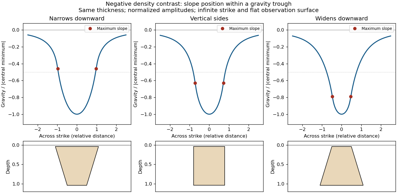

This qualitative inference assumes approximately comparable simple bodies, uniform geophysical density contrast, and a properly removed regional field. Gravity inversion is non-unique: lateral density changes, multiple bodies, and a buried top can imitate changes of wall slope. Use the seismic reflection constraints to test the interpretation.
Use the same surrounding basement density inferred in solution, carrying its unrounded value through the arithmetic. The intrusion's geophysical density contrast isThe Bouguer slab thickness needed to produce the same negative peak is thereforeThe smaller absolute geophysical density contrast requires a thicker body. This is an approximate vertical thickness and, if the top is close to the surface as drawn in Figure 1, an approximate base depth below that top. It is not an independent estimate of the intrusion's burial depth. For an infinite slab the anomaly does not depend on top depth; a buried top would require additional geometry. Finite width and the downward-widening outline in Figure 1 make 8 km a slab-equivalent estimate rather than a uniquely determined geological depth.
For a wide horizontal Bouguer slab replacing surrounding basement, use the density contrast , not the absolute sediment density:Take downward attraction as positive. The negative anomaly therefore requires . With , , and ,soThis is the requested Bouguer slab approximation: a flat observation surface, laterally infinite constant-thickness material, uniform average geophysical density contrast, and a regional anomaly already removed. The actual basin in Figure 1 narrows downwards and is finite. For a fixed maximum thickness, finite width reduces the central anomaly magnitude, so this calculation can underestimate the true magnitude of the average geophysical density contrast. It does not establish a unique basement density without the geometrical assumption.
A gravity anomaly is the difference between observed gravitational acceleration and a specified reference prediction after defined reductions. A free-air gravity anomaly, a Bouguer gravity anomaly, and a residual local gravity anomaly differ because they remove different reference contributions. State the reference ellipsoid, datum, reference density, and regional trend before interpreting an anomaly as a subsurface geophysical density contrast.
On land, tie gravimeter observations to a gravity base, calibrate them, correct instrumental drift and Earth tides, and determine station latitude and elevation accurately. Subtract latitude-dependent normal gravity . Reduce to the reference elevation using a positive free-air correction for a station above that datum: about for in metres. A simple Bouguer gravity anomaly then subtracts attraction of the intervening rock slab and adds the conventional terrain correction:with all acceleration terms expressed consistently. In SI units .
At sea, also correct vessel-motion effects, especially the Eötvös correction from east–west vessel motion and Earth rotation, and vertical ship acceleration; average or filter the moving-platform data appropriately. GPS navigation and tide information specify position and measurement height. Sea-surface measurements give a marine free-air gravity anomaly after motion, latitude, tide and height reductions. A marine Bouguer gravity anomaly additionally allows for measured bathymetry and the replacement of low-density water by reference rock; the simple water-column replacement correction is positive, , relative to the sea-surface free-air value. A consistent three-dimensional bathymetric correction is preferable near irregular coasts. Remove a justified broad regional field if the intended quantity is a residual anomaly of the local body.
A stability boundary in a mineral activity diagram must also be stable against the third mineral. Use the common-potential test for a three-mineral activity diagram. For the two corundum-producing directions,Negative values favour corundum. For the albite-to-nepheline conversion, , so low silica activity favours nepheline and high silica activity favours albite. These comparisons give:
All three coexist at the intersection. Pairwise mass-action equations alone do not distinguish the stable segments from their metastable extensions.
The net reaction quotient is when the solid and water activities equal one. Therefore its equilibrium line isa vertical line through the intersection of the other two. There is no dependence on , because the net reaction contains neither hydrogen ions nor sodium ions.
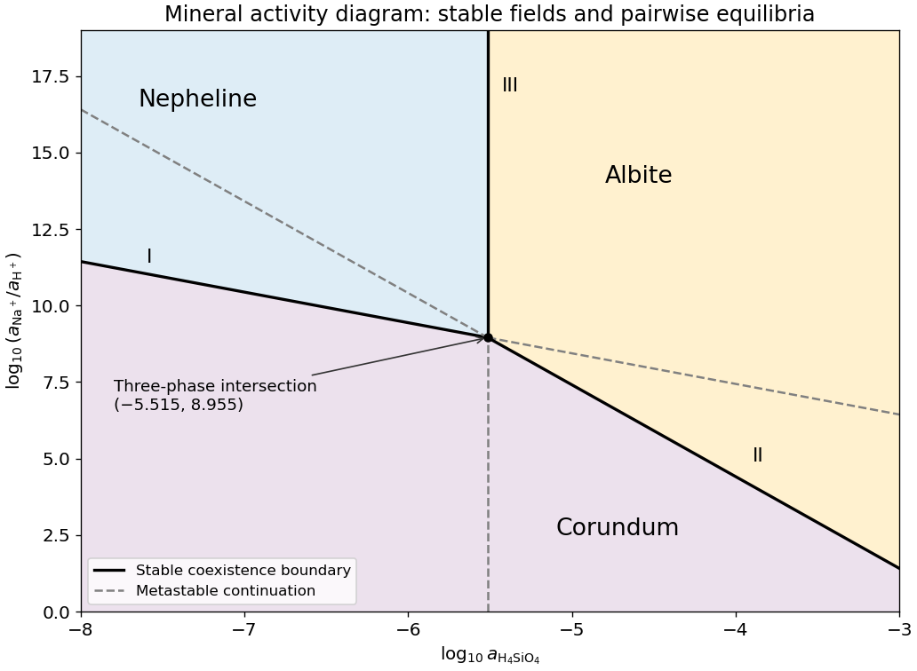
Stable and metastable mineral boundaries for the common albite-nepheline-corundum equilibrium example
. Original diagram computed from the supplied equilibrium constants. Solid lines show stable coexistence; dashed continuations are metastable. Logarithms are base ten. Details.
Subtract the nepheline–corundum reaction from the albite–corundum reaction and divide by two. In the albite-to-nepheline direction the resulting net reaction isAdditivity of the standard Gibbs energy of reaction makes the logarithms of the equilibrium constants combine with the same coefficients:This normalization is per one albite formula unit. The doubled reaction has , and reversing the reaction changes its sign.
Use base-ten logarithms and dimensionless thermodynamic activities at the stated temperature and pressure. Define and . The concentration notation is an ideal dilute-solution approximation with a consistent concentration reference.
With pure solids and unit water activity, the two reaction quotients are and . Equating them to the corresponding equilibrium constants givesThe slopes on the mineral activity diagram are and . The lines meet at , within the negative silica-logarithm range.
Use a high-resolution multichannel seismic reflection survey, with closely spaced crossing lines or a suitable small three-dimensional survey over the turbine locations. It should map the seabed, the sediment–sandstone boundary, local faults, buried channels, and lateral changes relevant to foundations. Seismic reflection responds to acoustic impedance contrasts and can image an irregular boundary without requiring it to be a first-arrival refractor. Here even the seabed has a useful normal-incidence reflection coefficient of despite its zero P-velocity contrast.
A seismic refraction survey can provide complementary seismic velocities and geotechnical information, particularly using seabed multicomponent receivers for S waves. Its limitations as the principal imaging method here include the missing water–sediment P refractor, required offsets of hundreds of metres to obtain useful basement first arrivals, and weaker constraints on thin layers or velocity inversions. Variable bathymetry and sediment thickness further complicate simple refraction interpretations.
A shallow-towed boomer seismic source or small sparker seismic source is a sensible initial seismic source for penetrating about 20 m of sediment beneath a 50 m water column. A chirp sub-bottom profiler can add finer imaging of the upper cover where penetration permits; penetration depends on grain size, consolidation, gas, and seismic attenuation. A pilot line should establish the minimum useful source energy and bandwidth. Large low-frequency air-gun arrays are unnecessary for this shallow target. Small coastal vessels, sea state, tow stability and acoustic background constrain usable frequencies and operations. Marine mammals and other local receptors motivate a low-energy effective source, monitoring and appropriate operational mitigation.[ref]
High-resolution multichannel seismic system by United States Geological Survey. The institutional instrument description lists configurable boomer, sparker, hydrophone-streamer and complementary chirp equipment for shallow subsurface mapping.
The expected normal-incidence two-way travel times are for the seabed and for basement, separated by . Source duration, recording sample interval and bandwidth must distinguish them. As an initial vertical seismic resolution estimate, : gives about in the sediment, although usable resolution depends on the whole seismic wavelet and signal-to-noise ratio.
Choose shot and receiver spacing from the shortest useful wavelength, target size, maximum reflector dip, seismic migration needs and achievable navigation accuracy. For a plane event of horizontal seismic ray parameter , avoiding spatial aliasing requires approximately . Source spacing and receiver spacing also set midpoint coverage and seismic acquisition fold; adequate offsets enable moveout correction and velocity estimation. For nearly horizontal shallow reflectors a few-metre shot interval can be practical, whereas steep events at high frequency require denser spatial sampling. These values must be designed together rather than imposing one spacing for every target. Cross-line spacing must resolve lateral features between turbine sites, not merely along each track.
At a vessel speed of , one shot per second gives 2 m shot spacing and ample separation relative to a roughly target return, subject to the longer record needed for seismic multiples and source recovery. Shallow towing limits seismic source ghosts and receiver ghosts, but requires stable tow depth. Accurate positioning, tides, measured water sound speed, bathymetry and checks for seabed seismic multiples are essential for correct target depths.
Take horizontal interfaces, water depth , and sediment thickness . Both source and receiver are just below the sea surface. Every angle below is measured from the vertical interface normal. Snell's law preserves the horizontal seismic ray parameterA basement seismic head wave of speed has horizontal propagation at the basement interface, so . The two possibilities are:
The water supports only P waves. At oblique incidence the seabed can convert a P wave into an SV-wave in the sediment, and the return SV-wave can convert back to a P wave in the water. Further seismic mode conversion can occur at the basement. Thus the down-going and up-going sediment legs can independently be P or S. The S entries refer to SV-waves; a fluid P wave source in this two-dimensional isotropic geometry does not excite the decoupled SH-wave sector.
Let be the distance travelled along the basement interface. For sediment legs ,The first-appearance distance is the limiting value at :
For example, the unconverted P branch gives . The earliest geometrically permitted basement P seismic head wave is the doubly converted path with sediment S legs, at approximately . The corresponding basement S family first appears at approximately . These limiting distances describe existence of ray branches; a finite detectable wave amplitude also depends on conversion efficiency and acquisition noise.
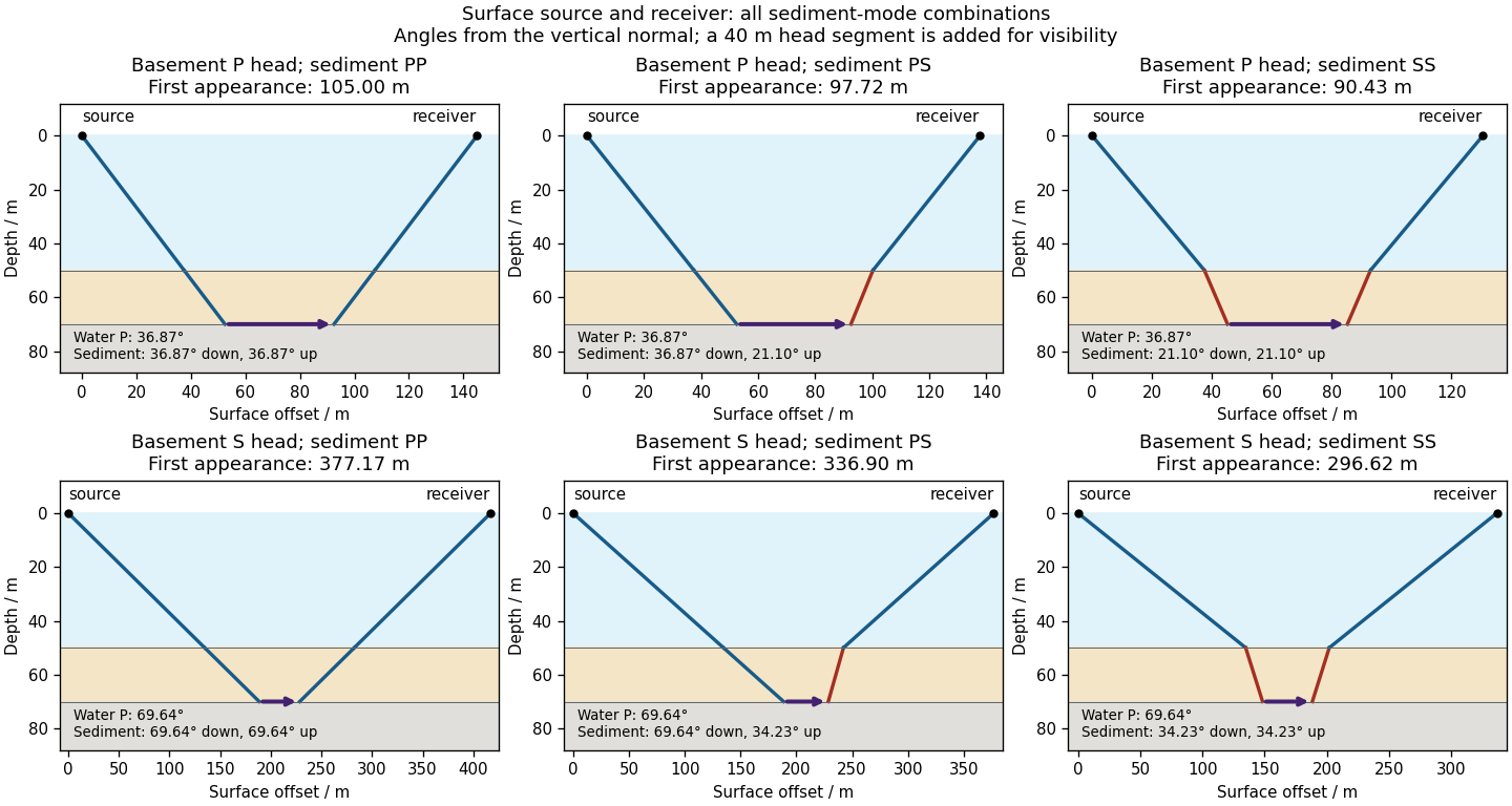

There is no separate finite-distance P head wave at the water–sediment interface: , so the nominal critical angle is , and a ray from a source 50 m above the interface cannot reach it at finite horizontal distance. Nor can the slower sediment S speed, , support a seismic head wave launched from water: it would require . A seismic reflection still exists at the seabed because the densities, hence the acoustic impedances, differ.
First appearance and first arrival differ. For each permitted branch the travel time isThe all-P basement P branch has . It overtakes the direct water P wave, , only at . The converted P-head branches have larger seismic intercept times, so even where they exist at shorter offsets they are later arrivals. The S-head branches are likewise later than the all-P P-head branch wherever they exist in this model. Reflections and layer reverberations can supply additional later phases.
The normal-incidence acoustic impedance is , with units . ThusDefine the pressure-amplitude reflection coefficient and pressure-amplitude transmission coefficient for incidence downwards from layer into layer byHere denotes compressional normal-stress amplitude; in the water it is the acoustic pressure. Continuity of normal traction and normal particle velocity gives these expressions. They describe each interface separately, before any layer layer reverberation.
For a lossless normal-incidence plane wave, intensity is proportional to , soA transmitted pressure amplitude exceeding unity is therefore compatible with conservation of energy. If instead the coefficient is defined for particle velocity measured along the same downward coordinate, and : the two transmitted velocity coefficients are and . Upward incidence reverses the sign of , interchanges the transmitted pressure and velocity coefficients, and leaves unchanged. At normal incidence between these ideal isotropic layers there is no P-to-S seismic mode conversion.
For an approximately isotropic rock, the P wave and S wave speeds arewhere is bulk modulus, is shear modulus, and is density. Five important controls are:
- Mineralogy and cementation. Stiff, well-cemented mineral frameworks usually have higher elastic modulus values and faster seismic velocities than poorly consolidated sediments. Density alone is insufficient: both stiffness and density enter the equations.
- Porosity and cracks. Larger porosity, especially compliant cracks, usually lowers effective elastic modulus values and seismic velocities. Crack orientation can make the seismic velocities direction-dependent through seismic anisotropy.
- Pore-fluid composition and saturation. Replacing liquid water by gas generally lowers the effective bulk modulus sharply and reduces . Pore fluids have negligible static shear modulus; responds chiefly through the solid framework and the changed bulk density, rather than through a shear restoring force in the fluid.
- Effective confining pressure. Increasing effective stress closes cracks and improves grain contacts, usually increasing both seismic velocities. Increasing pore fluid pressure at fixed total stress reduces effective stress and can reverse this trend.
- Temperature. At otherwise comparable conditions, increasing temperature generally softens minerals and lowers seismic velocities; thermal cracking or partial melting can lower them further. Increasing burial commonly increases both temperature and pressure, so their separate effects need not have the same sign.
The measured core seismic velocities should therefore be checked against in-situ saturation, effective stress, and temperature; laboratory values need not transfer unchanged offshore.
Four groups have pairwise comparisons. Testing each at test size without adjustment generally increases the familywise error rate, the chance of at least one type I error. If the six rejection events were independent, that chance would be ; shared samples make the actual comparisons dependent, so this expression is illustrative rather than exact.
A single omnibus ANOVA tests equality of all four means with one stated test size, avoiding that six-test inflation for the global question. If the aim is to identify differing pairs, follow with suitably adjusted comparisons, such as Bonferroni correction or a simultaneous pairwise method. A significant omnibus test does not automatically license six unadjusted claims. The benefit concerns control of type I error, rather than a guarantee that the model's independence and common-variance assumptions hold.
TODO: Attachment C is absent. Check its contents before treating this as a source-complete answer; the computation below uses the printed table, independent observations, a common within-season variance model and an explicitly chosen significance level.
For a one-factor analysis of variance, let be the four seasonal sizes, means and standard deviations. The weighted grand arithmetic mean isThis agrees with the rounded annual mean . The between-season and within-season sums of squares areThere are between-season statistical degrees of freedom, because the four fitted seasonal means are compared subject to their weighted grand-mean constraint. There are within-season statistical degrees of freedom, because one mean was estimated in each group. The total has , equal to their sum. HenceUnder , compare with the F-distribution on statistical degrees of freedom. The critical value is about , with p-value approximately from the rounded summaries. Reject equality of all four means very strongly under the stated model. The omnibus hypothesis test establishes that at least one mean differs; it does not identify every pairwise difference.
The summer variance is substantially lower than the other three, so the exact common-variance ANOVA assumptions deserve checking, as does temporal independence. Raw observations would permit diagnostics and a heteroscedastic or time-dependent analysis. As a cross-check on arithmetic, implies annual sample standard deviation , matching the table's . The numerical significance must not be mistaken for verification of the unobserved Attachment C or of the sampling model.
TODO: Attachment C is absent from the held release. Recover it to check any supplied critical-value table, significance convention or additional instructions. This leaf remains incomplete against that missing input. The printed summary statistics nevertheless allow the following conditional numerical answer, using a two-sided Student's t-test and independent observations with common variance.
Test against . The pooled sample variance isThe test statistic and statistical degrees of freedom areUsing the Student t-distribution directly gives a two-sided p-value and a critical value . Thus reject equal seasonal means at and ; the winter mean is higher by concentration units. This does not establish a large physical effect or its cause.
The two variances are similar, and Welch's t-test gives essentially the same result: , , . Both calculations assume the counts represent independent observations. Serial dependence, repeated measurements and strong non-normality can invalidate nominal p-values; the summary table alone cannot diagnose them. The unequal means are a conclusion under these statistical assumptions, pending recovery of Attachment C.
Squaring each seasonal standard deviation gives the seasonal variance in squared concentration units:
- Winter: .
- Spring: .
- Summer: .
- Fall: .
There are unlisted articles, also show them or only show them.