
Because , its even and odd powers are and . Separate the matrix exponential into these two power series:No representation of the gamma matrices is needed. Hermiticity of also makes this exponential unitary for real , while the projectors acquire opposite phases.
Contract the numerator of the quoted light cone gauge propagator with :Thus every internal gluon emerging from a ghost-gluon vertex contributes a factor . Every ghost-dependent contribution to a physical gluon or matter amplitude vanishes. Equivalently, the strict condition removes the Faddeev-Popov ghost interaction in i, leaving the field-independent determinant , which cancels from normalized correlators.
This is ghost decoupling in strict axial gauge, not a statement that the free Faddeev-Popov ghost propagator itself is zero. The algebra assumes a consistent axial-gauge pole prescription for and treatment of residual gauge zero modes. The overall sign assigned to the displayed vector propagator does not enter the contraction proof. With the mostly-minus convention and the usual action, its conventional prefactor is ; the source prints . Either prefactor gives the same zero contraction, so no sign correction is needed to obtain the requested ghost-decoupling result.
Choose an infinitesimal gauge transformation , where . Varying the axial gauge function at fixed givesThis is the Faddeev-Popov operator. The Faddeev-Popov determinant has a Grassmann representation . Choosing this normalization for the antighost givesA simultaneous antighost rephasing changes the overall ghost-action sign and vertex conventions, but not the determinant's field-dependent content. The essential facts are the kinetic operator and a ghost-gluon vertex proportional to .
Now average the fixed- constraint with the stated Gaussian:up to a field-independent normalization. ConsequentlyThe Faddeev-Popov ghost determinant is not generally field independent before imposing the strict axial condition: its interaction term contains . In the gauge this quantity vanishes on the integration slice, giving the decoupling established next. Defining the inverse of still requires boundary conditions for residual gauge transformations.
For two distinct commuting real scalar fields in place of the labelled fermion pair, with interaction , there is no anticommutation sign on closing the loop and no spinor trace. The two propagators are simply multiplied. In terms of physical time-ordered scalar contractions , the connected contribution isThe statistics and symmetry factors of a two-propagator loop determine the replacement. Relative to the fermionic formula in ii, the loop-statistics sign reverses. Scalar source kernels normalized like the stated Gaussian give the same overall minus sign after the four contraction factors are converted. There is no spin multiplicity.
If both replacement fields instead mean the same real field , the coupling normalization and the identical-line symmetry factor must be specified. With interaction , the cubic vertex is and its two-identical-line loop carries , giving coefficient . With the literal coefficient , its vertex is and the coefficient is . These cases are distinct from two separately labelled real fields; suppressing their combinatorics would hide a factor-of-two ambiguity in the replacement.
First fix the propagator kernels in a positive-sign Gaussian generating functional. From its scalar exponent, gives the contraction . The fermionic insertion rules similarly give , writing for the kernel labelled in that exponent. Thus the kernels in the question do not already include the factors of in the actual time-ordered contractions.
At order , expand the interaction operator to its second term, or equivalently apply Wick's theorem toFor a connected contribution, the external scalar insertions attach to different interaction points. The two assignments are equal after exchanging and cancel . The connected fermionic contraction isThe minus sign is the closed fermion loop sign. The alternative pairing gives two separate fermion tadpoles and belongs to disconnected external components, not the requested connected function. A free external scalar line multiplying a vacuum graph also cancels in the normalized result.
Combining with the loop minus sign givesThere are four contractions, so replacing and introduces . ThereforeThis is the fermion-loop diagram in the last panel of i. The trace contracts spinor indices around the loop; it is not an additional degeneracy factor. A convention using physical contractions directly obtains the preceding formula in with the same coefficient. Mixing one convention's Gaussian kernels with another's insertion factors would change its apparent signs.
Use the source action , with independent Grassmann variables used as sources and left functional derivatives. A scalar insertion is . For the odd fields the ordered rules areThe middle sign is not arbitrary: differentiating the rightmost odd source in from the left gives . Derivative ordering must consequently match the displayed order of the fields; the rightmost derivative acts first.
Expand in its power series. Replace each field in every term by its source insertion, preserving the fermion order. These derivatives can be pulled outside the free path integral. Re-exponentiation gives the unnormalized generating functionalSummation over the spinor index is understood. Normalized correlation functions require division by the same interacting , which cancels vacuum factors; that division is separate from this operator identity.
The double-longitudinal Ward identity for gluon fusion uses the defining Lie algebra identity makes the boxed amplitude vanish:In QED, both external gauge bosons are photons, the charge matrices commute, and there is no three-photon vertex. The two fermion-exchange graphs then cancel without a third graph. In QCD, omitting the three-gluon interaction would leave a generally nonzero colour commutator: gauge-boson self-interaction is essential to the cancellation.
This is a tree-level manifestation of a Ward identity and, more generally in a gauge-fixed non-Abelian theory, the Slavnov-Taylor identities. They connect the matter representation, the structure constants and the gauge interactions, ensuring that auxiliary longitudinal polarizations do not enter physical probabilities. With all other external legs physical and on shell, replacing one external massless gauge-boson polarization by its momentum leaves zero. The double-contraction result proved here is one consequence, not by itself a proof that every open-index amplitude tensor is transverse off shell. At loop order the corresponding non-Abelian identities also involve Faddeev-Popov ghosts and a consistent symmetry-preserving renormalization.
The tree-level Feynman diagrams are the two ordered quark-exchange graphs and the -channel gluon-exchange graph with a three-gluon vertex. There is no two-gluon-two-quark contact term in the ordinary QCD Lagrangian density. Let , , , and , , . Define as the product of the stated Feynman rules.
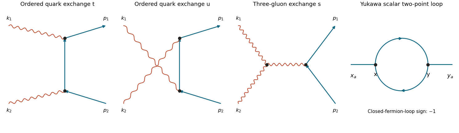
The three gluon-fusion tree diagrams and the Yukawa fermion-loop correction
. The first three panels show ordered quark exchange and three-gluon exchange. The last panel shows a directed closed fermion loop between two scalar insertions. Crossings without dots are not vertices. Details.
Suppressing external colour indices, the quark graphs areThe massless Dirac equations give and . ConsequentlyThe last equality uses . The quark-exchange sum is therefore .
For the gluon graph, use all incoming momenta in the three-gluon tensor:Its double contraction is . The vertex and gluon propagator giveCombining the graphs yieldsThus the requested spinor proportionality factor is when the colour matrix is displayed separately; retaining it inside the spinor bilinear makes its external colour indices explicit. For a convention calling the Feynman-rule product itself , rather than , the entire result gains one factor of .
Set the external four-momenta to zero after identifying the proper diagrams. In each box or triangle, at least one endpoint of the internal photon is a cubic vertex adjacent to an external scalar of zero momentum. That vertex is proportional to , whereas the supplied numerator obeys . All seven such graphs vanish algebraically. This use of the transverse numerator is stronger than merely saying that one has chosen a generic Lorenz gauge.
The two surviving seagull vertex bubbles have vertex factors and . Combining their two propagators givesThis scalar-QED four-point vertex pole in transverse gauge calculation determines the proportionality constant as well as the required tensor structure. Keep while extracting the ultraviolet pole. Lorentz covariance inside the regulated integral replaces by , giving the factor .
For its scalar integral, Feynman parameter givesThere is no infrared divergence at with nonzero . At pole order the two photon assignments and the factor therefore yieldThe common engineering scale factor is included in ; finite logarithms are immaterial to the pole. Adding cancels it whenThis is minimal subtraction scheme, up to optional finite terms. It agrees with the transverse-gauge scalar QED wave-function pole and . Setting at the outset would instead make the zero-momentum integral scaleless and obscure its separate ultraviolet divergence.
For the proper four-point interaction vertex, retain one-particle-irreducible Feynman diagrams with two labelled external photons and the two ends of a directed scalar line. Put for a cubic scalar–photon vertex and for a seagull vertex. The one-loop counting identities require . There are three possibilities, giving the nine proper scalar-QED seagull-vertex diagrams:
- Four cubic vertices: two box graphs, with scalar-line order or , where the end vertices are joined by the internal photon.
- Two cubic vertices and one seagull: one triangle with order , both external photons on the middle vertex; two with order , distinguished by which external photon is on the seagull; and two with order , with the same two choices.
- Two seagulls: two bubble graphs with order , distinguished by the external-photon assignment.
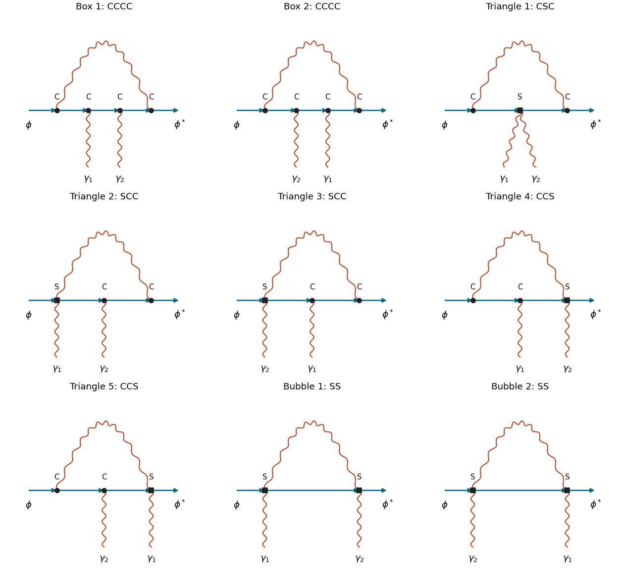

Each graph has Feynman-diagram symmetry factor one with these external labels: the internal photon and scalar are different species, and the charged scalar endpoints cannot be exchanged. The list is complete because the internal photon must join the ends of the open scalar chain for the graph to remain connected after any one internal line is cut. If it joined two interior points, an outside scalar segment would be a bridge and the graph would be one-particle reducible.
External-leg self-energy insertions contribute to an unamputated four-point correlation function, not this proper vertex. The local four-point counterterm from i is included separately when constructing the renormalized answer; it is not another one-loop topology. Abelian Faddeev-Popov ghosts do not interact in this linear gauge and add no diagram.
Let , , and define the renormalized coupling by . Write and . The complete renormalized Lagrangian density, with its counterterms already included, isSeparating off the classical renormalized terms leaves the counterterm LagrangianThe seagull vertex factor is thus . The bare covariant derivative fixes , rather than supplying an unrelated fourth charge parameter. The scalar QED Ward identity, for a symmetry-preserving regularization, gives and hence .
For an invertible quadratic gauge field operator, also include . One may choose , so this term needs no independent counterterm. The strict transverse limit is . Even if the renormalized quartic coupling is set to zero at one scale, its counterterm need not vanish: photon graphs generate a four-scalar interaction. The renormalized Lagrangian density must retain this allowed operator.
Since the hypercharge is zero, electric neutrality means . Choose the real-triplet vacuum , with . With canonical real-scalar kinetic density , insert this vacuum into the covariant derivative. The hypercharge field has no coupling to this scalar, while only are nonzero. ThusThe charged combinations haveBoth and the independent hypercharge generator annihilate the vacuum. The connected unbroken subgroup is thereforeThe electromagnetic generator belongs to it, but it is only one linear combination of two surviving neutral generators. This model has two massless neutral gauge fields, rather than the single massless photon and massive neutral vector of the usual scalar-doublet electroweak model. A neutral-field rotation does not create a massive eigenvalue from this zero block.
The two transverse triplet components are eaten, leaving one real, electrically neutral radial scalar . The radial eigenvalue of the Hessian found in part i isIndeed the radial potential is a constant plus , fixing the factor of two between its quadratic coefficient and its mass squared. The physical degree-of-freedom count is preserved: three real scalars plus four massless vectors give , while one scalar, two massive vectors and two massless vectors give .
Gauge invariance of the scalar potential implies the infinitesimal identityThe irrelevant common factor from the real representation's infinitesimal rotation has been divided out. Differentiate with respect to and evaluate at the stationary vacuum :The second term vanishes by stationarity, leavingWhenever , this is a nonzero vector in the kernel of the scalar mass-squared matrix, so it is a zero-eigenvalue direction. It is tangent to the degenerate vacuum orbit. In a global theory it is a Goldstone direction; in the gauged theory the corresponding would-be Goldstone field supplies a longitudinal polarization of a massive vector.
For the specific potential, stationarity at a nonzero vacuum gives , assuming and . Its Hessian isThe antisymmetry of the triplet generators gives , verifying the claimed kernel directly.
For the ghost coupling in a linear Cartesian Abelian Higgs gauge, the common factor in the scalar parametrization cancels from the gauge transformation. Separating real and imaginary parts givesConsequentlyFor the variables and gauge function actually printed, the ghost mass and Higgs-ghost vertex are thereforeFor the usual nonnegative gauge parameter, . The momentum-space ghost propagator is in this kinetic convention. There is no direct ghost-photon vertex or ghost- vertex. At the ghost becomes massless and decouples.
The scalar prefactor is incompatible with the stated canonical broken-vacuum interpretation. At it gives , whereas the potential is minimized at . In fact the printed parametrization givesIts kinetic terms have coefficient , not , and its vector mass parameter is . The given gauge function consequently does not cancel the vector-scalar mixing in those literal variables. The ghost operator computed above nevertheless follows algebraically from that gauge function without changing the printed fields.
With a canonical Abelian Higgs shift , the expansion is about a true minimum, the vector mass is , the gauge fixing cancels the mixing, and the same ghost formulas acquire the usual interpretation . For the literal parametrization, a canonical fluctuation is , so its ghost vertex would instead be ; the non-vacuum background problem still remains. These two interpretations must not be silently mixed.
The gauge-invariant functional integral counts every gauge orbit repeatedly. Insert a gauge-orbit identityDividing by the gauge-group volume and averaging with a Gaussian weight produces the term . The determinant is represented by a pair of independent anticommuting scalar fields , giving the prescribed ghost density , where . The Grassmann integral gives a determinant rather than the inverse determinant of a commuting Gaussian integral; field-independent constants and overall determinant signs are absorbed in normalization.
Although the gauge group is Abelian, the determinant here is field dependent because the gauge condition contains the scalar fluctuation . Thus Abelian ghosts need not decouple in a broken-phase gauge. The fields implement gauge-orbit counting and are not physical external particles.
Continue with and dot products in that auxiliary metric. Odd gamma traces vanish. The two current tensors areContracting givesLet . The on-shell products are , , and . Substitution yieldsThe result is already averaged over incoming colours and spins and summed over outgoing ones. For , it becomes .
The different-flavour quark annihilation into a massive pair has only an -channel gluon graph at tree level when the two quark flavours differ. Its amplitude contains one incoming and one outgoing colour current, with common magnitude factor . On-shell current conservation removes the gauge-parameter-dependent longitudinal part of the gluon propagator. To display the Dirac signs transparently, evaluate spin traces with the auxiliary mostly-minus metric and ; the invariants are then the usual positive-energy Mandelstam invariants, numerically identical to those defined in the paper.
The incoming colour average and outgoing colour sum giveAveraging over the two spins of each incident particle supplies an additional . The physical spin sums are and . ThereforeThe coefficient is equivalently , with .
The two top projectors cannot both contain . The printed expression has that error. It is not repaired by changing the metric convention consistently: a particle and antiparticle still require the appropriate distinct projectors. In the auxiliary convention, its outgoing tensor would obey , rather than zero for . At threshold it gives a zero contracted trace, while the correctly averaged vector-current production amplitude squared has a nonzero limit . The phase-space cross section still vanishes at threshold because the final velocity tends to zero. The colour and spin prefactor above is consequently the prefactor for the corrected trace; no overall constant can make the misprinted massive trace the physical answer for all kinematics.
At first order the Dyson expansion inserts . Contract the scalar field at the vertex with the external scalar. The four remaining fermion fields have two admissible pairings: both external fermions attach to the vertex, or the two vertex fermions contract with each other while the external pair contracts freely. Wick's theorem givesThe minus sign in the second term is the fermion sign of the closed contraction: . The first term is connected; the second is a scalar-attached fermion tadpole multiplied by a disconnected free external fermion propagator. The full time-ordered expectation includes both topologies, whereas the connected generating functional retains only the first. There is no order- contribution in this pure Yukawa expansion because the total number of scalar fields would be odd.
For a parity-preserving free propagator, the tadpole coefficient is , whose integrand contains only and . Both vanish. Thus the second term is a legitimate formal Wick contraction but is zero with a compatible regulator; normal ordering the interaction removes it from the outset.
Use the source term and left Grassmann functional derivatives. Differentiating its exponential inserts fields according toThe sign for follows because a left derivative with respect to must cross . Keep the order when replacing these fields. Expand in the original path integral; each field monomial can now be generated by these ordered derivatives acting on the free functional. Resumming givesThe arguments refer respectively to at . The free functional arises by performing the free Gaussian field integrals, and may be chosen so that .
No additional field-integration measure remains in this differential-operator formula. Such a measure is printed outside the operator in the source even though has already integrated out those fields. At , that literal expression would contain rather than simply , which is not the free generating functional. Also, when denotes a density, the spacetime integral in the exponent is required.
Use the fundamental SU(3) normalization , with Hermitian generators. The average over the incoming colours and sum over the outgoing colours givesThe complete spin and colour averaged result is consequentlyFor massless two-body centre-of-momentum kinematics, and , so the same answer is . This checks positivity, the symmetry under exchanging the outgoing directions, and the absence of a forward -channel singularity in this particular process.
There are unlisted articles, also show them or only show them.