Equilibrium emittance obeys ϵx=Cqγ2I5/(JxI2), with I5=∮H(s)∣ρ∣−3ds, H=γxη2+2αxηη′+βxη′2. Thus reduce both bend angles and the dispersion invariant inside bends, rather than merely focusing to a small beam size elsewhere. The damping partition can also be adjusted within stability constraints.
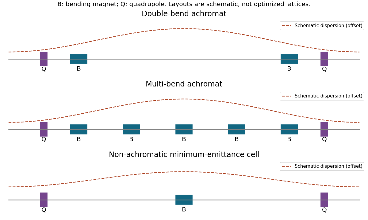
A DBA uses two bends and quadrupoles to return dispersion and its slope to zero at the cell boundaries; this provides dispersion-free insertion straights, at some emittance cost. A multi-bend achromat distributes the total angle over more weak bends and carefully controls the interior dispersion. A non-achromatic theoretical-minimum-emittance cell permits nonzero boundary dispersion and chooses the beta function and dispersion near a bend's optimum; longitudinal-gradient or reverse bends offer further control of radiation integrals. Strong focusing and dispersion suppression can increase natural chromaticity and sextupole demands, compromising dynamic aperture and momentum acceptance.
Doubling the number of identical-angle bends halves each angle. The minimum emittance scales as θ3, so it becomes 0.240nmrad. At unchanged energy and unchanged individual magnetlength, the bending radius doubles and field halves, giving B=0.70T and Ec≃4.19keV.
At fixed stored current the loss per turn, proportional to E4∮ds/ρ2, halves: twice as many equal-length bends each have one quarter of the original contribution. Total radiationpower therefore halves. The spectrum softens by the factor-two critical-energy change. The characteristic high-energy vertical opening angle remains of order 1/γ at fixed energy, while each magnet's horizontal sweep halves. At a fixed absolutephoton energy the normalized spectral position changes, so a claim that every angular distribution is identical would be too strong. Lower emittance also reduces the electron source size/divergence subject to the optical functions.
For identical uniform bends in an ideal double-bend achromat, the standard minimum is ϵx,min=Cqγ2θ3/(415Jx), with bend angle θ=2π/48 and γ≃3000/0.511. Hence ϵx,min≃1.92nmrad. This uses the achromat constraint; the unconstrained theoretical-minimum-emittance coefficient is three times smaller.
For fixed quadrupolefields and fractional momentum offset δ, q(δ)=q0/(1+δ). Differentiate cosμ=1−L1L2q2/2 at zero to obtain dμ/dδ=−L1L2q02/sinμ=−2tan(μ/2). Thus
Both transverse planes have the same natural result; the ring value is Ntimes this. It vanishes only in the zero-focusing limit, outside robust stable operation. Additional correcting elements, such as sextupoles where dispersion is nonzero, are required for zero corrected chromaticity.
The zero-strength endpoint is only marginal and usually gives a drifting Jordan block. The phase advance increases from zero to π on the positive-strength stable branch. Repeating the cell Ntimes gives ring eigenvaluese±iNμ and tune Nμ/(2π); it does not enlarge the stable strength interval. Integerring phase advances can be resonance-sensitive in the presence of errors even when the ideal repeated matrix is bounded.
Take areference point immediately before the focusing quadrupole and let matrices act on (x,x′) from the right. With q=1/f, define QF=(1−q01), QD=(1q01) and D(L)=(10L1). One cell is
Its determinant is one. A different starting point gives a conjugate matrix with the same trace and stability; the orthogonal transverse plane replaces q by −q.
where the spin projection is aligned with the charge-fieldsign. For spin one the lowest aligned mode has E2=m2c4−∣e∣ℏ∣B∣c at pz=0. Above ∣eB∣>m2c3/ℏ, this is negative: linear timeevolution has exponentially growing/decaying modes, signaling an instability of the assumed background.
Spin alone does not fix a magnetic moment. The scalar and Dirac examples cannot establish this formula for every higher-spin particle; the stated instability belongs to the specified g=2fieldmodel and its regime of applicability. Interactions and backreaction are needed to describe its eventual outcome.
For B>0 the two spinsigns are equivalently m2c4+2mc2[pz2/(2m)+μB(2n+1)±μB]. Both positive and negative relativistic energy branches arise from this squared equation; an actual Dirac spinor must still be reconstructed from the coupled equations, especially at exceptional values where division by E+mc2 is unavailable.
If the source's variable ξ=(pxc+eBy)/(ℏc)=bBY is used literally, bB=eB/(ℏc), then the same canonical oscillator form has M=m/bB2,ω=ωc and the same ε. Because ξ is an inverse length, this auxiliary M is not a physical particle mass with ordinary mass dimensions; the rescaling must be carried through both kinetic and potential terms.
Eliminate the lower component to get (E2−m2c4)φ=c2(σ⋅Π)2φ. Since [Πx,Πy]=ieℏB/c, the Pauli identity gives (σ⋅Π)2=Π2−eℏBσ3/c. Substitute the three momenta and rearrange:
The chosen gauge is independent of x,z,t, so simultaneous energy and canonical px,pzeigenstates justify the exponential ansatz. On the remaining spinors use Πx=px+eBy/c, Πy=−iℏd/dy, Πz=pz. The coupled equations are (E−mc2)φ=cσ⋅Πχ and (E+mc2)χ=cσ⋅Πφ.
Rewrite the real-energy probabilityas T=[1+U02sin2(ζa)/(4E(E+U0))]−1. Thus Tmax=1 at ζa=jπ, namely Ej=ℏ2j2π2/(2ma2)−U0≥0, with a strictly positive resonanceenergy in the ordinary scattering problem. Between resonances it is less than one and its oscillations approach one as energy increases. Generically T(0+)=0; a well tuned to a zero-energy resonance instead has T(0+)=1. The original transmission plot in S1 illustrates these maxima for a chosen well, not a universal specified depth.
For the amplitude continue to k=iκ on the decaying physical sheet. Then ζ=q and D=cos(qa)+(κ2−q2)sin(qa)/(2κq). The double-angle identity factors its zero condition into the even and odd matching conditionsκ=qtan(qb) and κ=−qcot(qb). Thus physical upper-half-planeamplitudepoles are exactly the bound energies.
The literal statement for the probability requires correction. The displayed real-axis expression continued algebraically is 1/[D(k)D(−k)], and includes poles of the opposite-boundary-condition amplitude too. A concrete counterexampleuses ℏ2/(2m)=1, a=2, q=1, κ=cot1 and U0=1+cot21. Its continued probabilitydenominator vanishes at k=icot1, because D(−k)=0. But neither κ=tan1 nor κ=−cot1 holds, so E=−cot21 is not a bound energy. Keeping the amplitude and the decaying boundary condition removes this spurious identification.
Continuity has already been built into these forms. At b, derivative continuity requires −qsin(qb)=−κcos(qb) for even parity and qcos(qb)=−κsin(qb) for odd parity. Thus
Use q/κ=U0/∣E∣−1 to obtain the two printed equations. The right side is positive, so only the corresponding allowed tangent/cotangent branches can describe a bound state; squaring without retaining this sign restriction adds spurious roots.
The respective inverse squared normalization constants are b+sin(2qb)/(2q)+cos2(qb)/κ and b−sin(2qb)/(2q)+sin2(qb)/κ. These include both exponential tails.