The cylindrical part has length2 micrometres and radius0.5 micrometres. Including both hemispherical ends gives area A=2πrL+4πr2=3π×10−12m2. The membrane capacitance is C=ϵ0ϵrA/d≃4.17×10−14F. Define the signed inward electrochemical drop per unit positive chargeas
There is a factor-of-two ambiguity in the wording of the chargedata. If the stated excess means the inner capacitorchargeQ=−40000e, then Δψ=Q/C=−0.154V and Δp≃−0.183V at 298 K. If “inside minus outside” is taken literally as Qin−Qout=−40000e for opposite capacitorcharges, the inner plate has −20000e, giving Δψ=−0.0768V and Δp≃−0.106V. The latter is the literal charge-difference interpretation; the former is the commonly intended excess-charge convention. In either case inward protonmotion is favorable, and the positive available driving magnitude is −Δp.
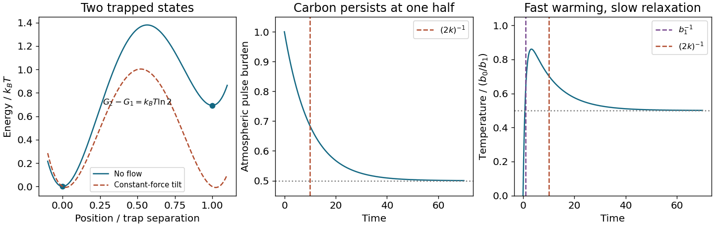
In a sufficiently uniform flow the Stokes force is F=γv toward trap 2. Its work over separation d lowers the second effective well by Fd. Equal effective freeenergies require γvd=kBTlog2. Hence
The sketch has two wells separated by 1 micrometre, with the secondfree-energy level higher by kBTlog2 and an intervening escape barrier. Free energy includes the volume of each trapped basin; equal minimum potential heights alone would not ensure equal occupations if basin shapes differed.
Write the displacement after m independent isotropic zero-mean steps as R=∑jsj. Cross terms vanish, giving ⟨R2⟩=mΔ when Δ=⟨∣s∣2⟩. Isotropy makes each Cartesian variance one third of this. Since m≃kt and ⟨R2⟩=6Dt, D=kΔ/6. If “step size” were instead defined asa single-coordinate mean square, the corresponding expression would be kΔ/2; the factor of three is purely the stated three-dimensional convention.
At 298 K with a=0.5μm, this gives approximately 4.37×10⁻¹³m2s−1. The argument assumes an overdamped particle in an equilibrium thermal bath, rather than arbitrary driven diffusion.
To pass to a↓0 without an invalid dominated-convergence argument on an infinite interval, pair positive and negative xfirst: the imaginary part is odd and the real part is 2∫0∞xsinx/(x2+a2)dx. On a bounded interval the limit is harmless, while integration by parts bounds the oscillatory tail uniformly for 0<a≤1. This gives the convergent improper Dirichlet integral∫−∞∞sinx/xdx=π.
Its interior poles are zero and r=−1/(1−2i); the other quadratic root is −5/(1−2i) and lies outside. The residues are 1/[i(1+2i)] and (r2+1)/(4ir), whose sum is i/10. Consequently
As an independent generating-function check, F(s)=∫0∞xs/(1+x2)dx=π/[2cos(πs/2)] for ∣Res∣<1. Differentiating twice and four times at zero gives the same moments.
The Ij are real and convergent. Comparing real and imaginary parts proves I0=π/2,I1=0. Independently, x↦1/x changes the sign of each odd logarithmic moment and preserves the measure, so every odd Ij vanishes.
The large circle contributes O((logR)n/R) and the small circle contributes O(ϵ∣logϵ∣n), so both disappear. The enclosed simple poles are i and −i, with logarithmsiπ/2 and 3iπ/2. Their residues are (iπ/2)n/(2i) and −(3iπ/2)n/(2i). The positive orientation of the keyhole therefore gives
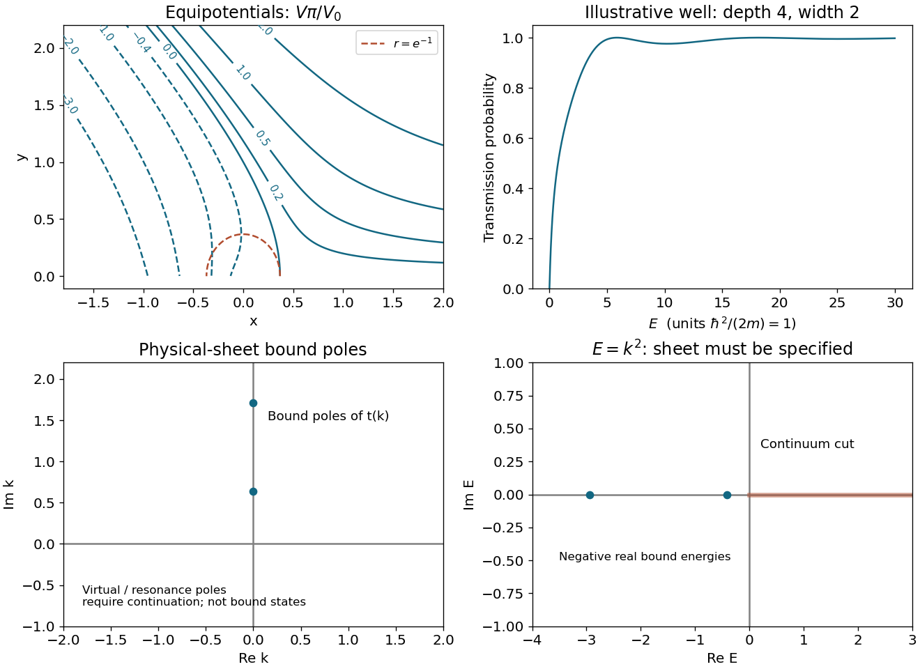
In the intended upper half-plane0<θ<π, the slope is positive for 0<r<e−1, vertical at r=e−1, and negative for r>e−1. At the positive real boundary θ=0 the slope is zero except at the stationary point(e−1,0), where both derivatives vanish and the quotient is indeterminate. More generally, outside the chosen half-plane its sign is the sign of −θ(1+logr), with the argument branch held fixed. A convenient parametric description of the curves to sketch is Vπ/V0=r(sinθlogr+θcosθ).
For the upper half-plane use 0<θ<π, and interpret the source's arctangentas this argument. Then V=(V0/π)Im(zLogz) is harmonic, so E=−∇V has zero curl and divergence where there is no charge. On the positive boundary θ→0 and ylogr→0; on the negative boundary θ→π. Hence the two boundary values are respectively zero and V0x.
Lossless Hamiltonian focusing can reduce a beam's transverse position width at the expense of momentum spread, but cannot reduce its occupied canonical phase volume. Coupling to the longitudinal direction can redistribute projected emittance without reducing total emittance. True cooling requires exporting entropy to additional degrees of freedom or discarding particles: stochasticfeedback, electron cooling or radiative damping coupled to an external environment provide possible mechanisms, with very different efficiency for high-energy protons. Collimation shrinks the accepted distribution at the cost of intensity. Acceleration also reduces angular divergence at fixed normalized emittance, an apparent geometrical cooling rather than a violation of Liouville's theorem. The apparatus and radiation cannot be omitted from the accounting when the bunch is no longer an isolated Hamiltonian subsystem.
Its determinant is cos2ωt+sin2ωt=1, explicitly preserving area. The orbits are energyellipses; stretching one coordinate during transport is compensated by the conjugate direction.