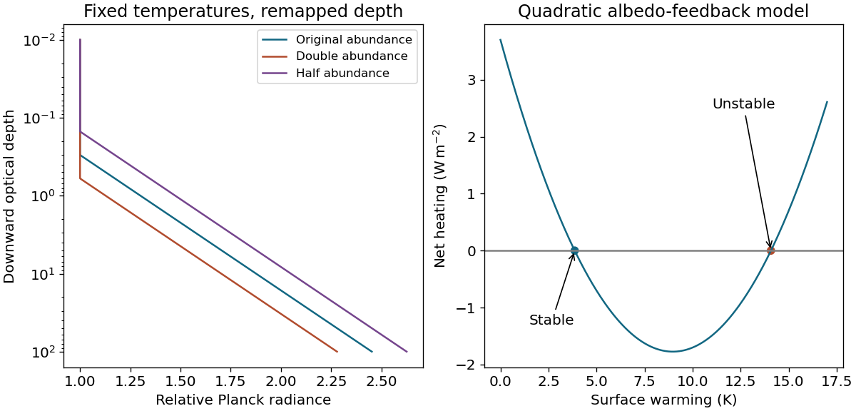
It is constant in the isothermal stratosphere and rises linearly with logτ below it. At unchanged temperatures and a multiplicative abundance change a, optical depth at each height changes to aτ, hence Ba(τ)=Bold(τ/a). Doubling moves the tropopause kink to 2τt and gives colder emission temperatures at a fixed optical depth; halving does the opposite.
Each layer emits in proportion to Bdτ and is attenuated by its overlying optical depth. The normalized exponential weighting emphasizes optical depths of order unity, while retaining contributions from a range of heights.
This compares matter specifically with the supplied CMB photons. Adding relativistic neutrinos changes the total radiation equality redshift; it is not included in these data.
Choosing the Big Bangas t=0 yields R=(t/t0)2/3 and H=2/(3t). Consequently t0=2/(3H0)≃9.3Gyr for the supplied H0. This is the age of the flat pressureless model without a cosmological constant, not adetermination in the current multi-component cosmological model.
At a fixed cosmological time, homogeneous expansion has v=H(t)r. A comoving galaxy has r=R(t)x with constant x, hence v=R˙x=(R˙/R)r. Thus H=R˙/R. Peculiar velocities must be removed before applying this ideal relation to individual galaxies.
For this cool giant, line blanketing and molecular absorption substantially distort a simple continuum peak, so Wien'slaw is the least reliable of these approximations. A detailed spectroscopic analysis, checked against a multi-band atmosphere fit, would generally be the strongest of the three if gooddata and modelparameters are available. There is no unconditional accuracy ranking without measurement errors and model systematics; an accurately measured angular diameter plus bolometric flux would offer a more direct effective-temperaturedetermination, if obtainable.
This is a cool luminous giant, in the red-giant region of the Hertzsprung-Russell diagram. On the usual first-ascent interpretation, luminosity comes predominantly from hydrogen shell burning around an inert helium core, with gravitational adjustment also contributing. The two measured quantities alone do not uniquely determine evolutionary history: a later giant phase can overlap this region, so they do not prove the precise core-burning state.
The angular radius follows directly from a(AU)/d(pc). Taking α=4 changes these estimates by only a few percent, but the calibration must be stated. Hubble's2.4maperture has visible-lightdiffraction scale 1.22λ/D≃0.05 arcsec at 500 nm, hundreds of times larger. The separation is therefore unresolved even before the severe star/planet contrast is considered.
Thus Mp3≃PVs3Ms2/(2πG) when Mp≪Ms. For a non-edge-on orbit the measured velocity instead determines Mpsini to this accuracy; neglecting eccentricity is also part of the stipulated model.
In the cold underdense model, 1−vg/c≃n/(2nc) and γϕ2≃nc/n=500. A relativistic electron slips through half an accelerating sinusoidalwavelength over Ld≃γϕ2λp≃8.35 mm. For Ez=E0sinϕ and injection at the start of that half-cycle, integration over 0<ϕ<π gives
For linear polarization, a0=eEL/(mecω0) and I=ϵ0cEL2/2. Substitution gives a0≃0.855λμmI/(1018Wcm−2)≃0.64. Thus the specified peak electronquivermotion is at most mildly relativistic, not highly relativistic. Its quiver Lorentz factor is of order 1+a02≃1.19. The supplied 40 TW fixes a focal area through P/I, but does not increase a0 once the intensity is specified. This exposesa limitation of assuming a strongly nonlinear, fully wavebreaking wake in the preceding estimates.
The laser driver should occupy at most roughly half a plasma period to excite the accelerating density response effectively. Interpreting pulselengthas full significant spatial duration gives ℓmax∼λp/2≃8.35μm,τmax∼27.8fs. If the source's σ denotes the rms width of a Gaussian envelope instead, the resonant scale is commonly kpσ∼1, or σ∼2.66μm and 8.9fs; full duration and rms width cannot be assigned the same numerical value without apulse-shape convention. The robust condition is a sub-plasma-period pulse.
The cold relativistic field scale is E0=mecωp/e≃1.92×1011Vm−1, corresponding to an energygradienteE0≃192GeVm−1. It is an upper scale for the stipulated large-amplitude wave, not proof that the particular weak driver produces that field.