
Apply the Leibniz rule to the th derivative in Rodrigues' formula. If derivatives fall on and on , the corresponding term is . Cancelling the prefactor givesThe leading coefficient is nonzero, so this is a polynomial of degree exactly . In particular, the requested coefficients in areThese are the ordinary Laguerre polynomials, with normalization .
Simplify the real component to . Thus is the unit circle with excluded from the mapping's domain. Its upper semicircle has and its lower semicircle has ; the point maps to . Inside the disk, , so the principal arctangent is unambiguous. Setting givesThe Laplace equation follows from (b). Approaching an open upper boundary arc makes the ratio tend to , giving ; the lower arc gives . This solution is in terms of the harmonic measure of a semicircle in a disk .
The boundary data jump at , so no path-independent continuous boundary value can be imposed at those two junctions. The displayed bounded harmonic function is the solution with the specified limits on the open arcs; those endpoint discontinuities are part of the idealized capacitor geometry.
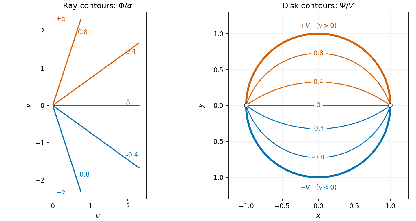
Harmonic ray contours in the right half-plane and the potential in a disk with opposite semicircle boundary values
. Details. 
Let . Direct partial differentiation, away from , givesThese are the Cauchy-Riemann equations. Equivalently, with , the analytic mapping is , the inverse Cayley transform between the half-plane and disk.
The supplied harmonicity result can also be checked by the multivariable chain rule. The Cauchy-Riemann equations imply , , and . HenceThis is conformal invariance of harmonicity for the given mapping.
Put . In the right half-plane,The last two cancel, so . The possible singular point lies outside the open domain .
For , a level curve of value has . These are rays from the origin, restricted to the right half-plane. For positive , the values increase with angle from on the lower boundary to on the upper boundary. If , the function is identically zero. The left panel of the figure in (c) shows these ray-shaped level curves.
The lazy choice weights are and , in ratio three to one. Normalizing gives . Let denote selection of the first question and let . Its conditional expected value, divided by , isso . If the overall lazy fraction is , the law of total probability gives . Bayes' theorem then givesSolving yields . The observed mean is conditioned on the chosen question, so it cannot be equated directly to the unconditional mean over all students.
Temporarily label the individual pieces. A random placement is a uniform injection of thirty-two distinct pieces into sixty-four squares, giving equally likely outcomes. For a colour-matching placement, the black pieces have available injections, and independently the white pieces have the same number within their disjoint set of squares. ThereforeHere . Treating same-colour pieces as indistinguishable gives the same probability, because the common within-colour labeling factors cancel. The two colour choices in the favourable count occupy disjoint square sets; no independence assumption about unrestricted placements is required.
For small , the binomial series gives the uniform expansion . Since , integration yieldsAlso , so the familiar symmetric approximation is equivalent to this order. This is the first correction in the ellipse perimeter expansion near a circle; the two approximate formulas need not agree at order .
Differentiating the parametrization gives and . Thus the arc length element isAll four quadrants give the same contribution. Consequently the ellipse perimeter isThe final factor is the complete elliptic integral of the second kind, evaluated at the eccentricity of a conic .
Use the integration by substitution , with . On this interval , so it cancels the positive denominator square root. The transformed integral isIts integrand is even. Therefore the answer in the PDF's modulus-amplitude convention for the elliptic integral of the second kind isThe modulus is , not the squared parameter .
If , the first formula in (a) gives andSubstitute this and into :For finite physical times , the domain is , valid for either sign of . If , the trajectory is vertical, , and in general no single-valued graph describes it. As a consistency check, the logarithmic expansion at fixed cancels the apparent terms and gives as , the drag-free parabola.
First solve for the velocity components. The integrating factor givesIntegrating once more and imposing the initial position givesThese formulas describe projectile motion with linear drag. Differentiation checks both second-order differential equations and both initial velocities. At large positive time, the horizontal velocity tends to zero and the vertical velocity tends to the terminal value .
There are unlisted articles, also show them or only show them.