
Factor . This givesThe last function is even. Its Taylor series begins , since and . ThereforeIn particular, the cubic coefficient is zero; the identity explains its cancellation before any lengthy differentiation.
The required derivatives are , , , and . The four-term Taylor polynomial about one, evaluated at two, isThe Taylor remainder is for some . ThusIts negative sign also shows that this approximation is an overestimate. Bounding the fourth derivative throughout the interval establishes the requested error estimate without using a decimal value of .
A cubic version of Taylor's theorem requires the corresponding higher differentiability, rather than only one derivative. For example, if has four continuous derivatives on the interval between and , thenwhere the Lagrange form of the Taylor remainder isfor some strictly between and when they differ. At , the remainder is zero. These hypotheses apply to both functions used below.
With , integrate the coefficient with respect to :Its other partial derivative is . Matching the coefficient gives . Therefore the differential equation is , and its implicit general solution isThese are level curves of the potential of a conservative vector field. Where , they give the usual graph solution . At , the implicit description retains possible vertical tangents instead of dividing by zero.
Write the differential one-form as . An exact differential form must satisfy equality of mixed partial derivatives, . HereEquality at every holds precisely when . Since these polynomials are smooth on the simply connected plane, the closed-form condition is also sufficient for exactness; the explicit potential of a conservative vector field constructed in (c) verifies that sufficiency directly.
The multivariable chain rule givesSubstituting the three parametrizing functions also writes the complete derivative asAt , the point is , its velocity is , and . Hence
The condition at infinity gives . Matching the electric potential at givesConsequentlyThis function is finite and differentiable at the origin. At the joining radius, both and match, giving and . Thus the electric field is continuous there as well as being conservative on each side. This is the potential of a uniform spherical source, with source coefficient .
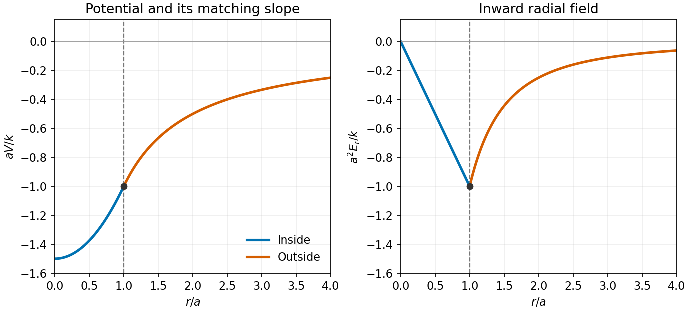
Continuous radial potential and inward electric field, normalized at the sphere boundary
. Details. 
For a radial electric potential, . Comparing radial coefficients givesIntegrating these one-variable derivatives gives the general local expressionsThe two constants are initially independent because these integrations were performed in separate radial regions.
Inside the sphere, the electric field has the form , including at the origin. Thus it is a conservative vector field. Outside, use the gradient of a radial function to obtainThis is also an explicit potential of a conservative vector field, single-valued throughout the exterior region. Equivalently, the curl vanishes in both regions: for a radial coefficient , because is radial. The interior formula avoids any apparent issue at the origin. The vector-field potentials here have the opposite sign from the electric potential convention used in (b).
The volume of a parallelepiped is the absolute scalar triple product of its three edge vectors. Since ,The factor appropriate to a tetrahedron must not be applied to this parallelepiped.
The characteristic equation factors as , giving . The superposition principle lets us find particular solutions for the two forcing terms separately. A trial gives and , so it is . A trial gives , so . Therefore
The characteristic equation has the repeated root . Its homogeneous solution is therefore . For a particular solution, try . Substitution gives , so and . Thus the general solution isThe extra factor in the second homogeneous term is required by the repeated root.
The characteristic equation is , giving . The initial conditions give and . Solving yields , , henceThe two distinct characteristic roots supply all solutions of this second-order linear ordinary differential equation.
Subtract the integrands first, using . Then set :The further integration by substitution makes , soThis also holds at .
Apply the power-complement integral recurrence three times, starting from :Each factor corresponds to reducing by one; the final unreduced integral is just .
Set , so , and write . The integration by substitution gives . For , integration by parts yieldsBoth endpoint terms vanish. Use inside the remaining integral:ConsequentlyThis is the instance of the power-complement integral recurrence, with initial value .
Apply the fundamental theorem of calculus separately to the upper and lower limits. No evaluation of the integral is needed:The first result has no dependence and the second no dependence, so the mixed partial derivative is
There are unlisted articles, also show them or only show them.