
Real coefficients imply that the conjugate is also a polynomial root. Write the remaining root as . ThenThe coefficient of in this product is . That coefficient is zero in the specified polynomial, so . Hence the two other roots areAs a check, the full polynomial is , corresponding to , and .
The original PDF asks for cube roots of . Their complex modulus is , and their arguments are , . Converting to Cartesian form givesCubing any one gives the positive real number .
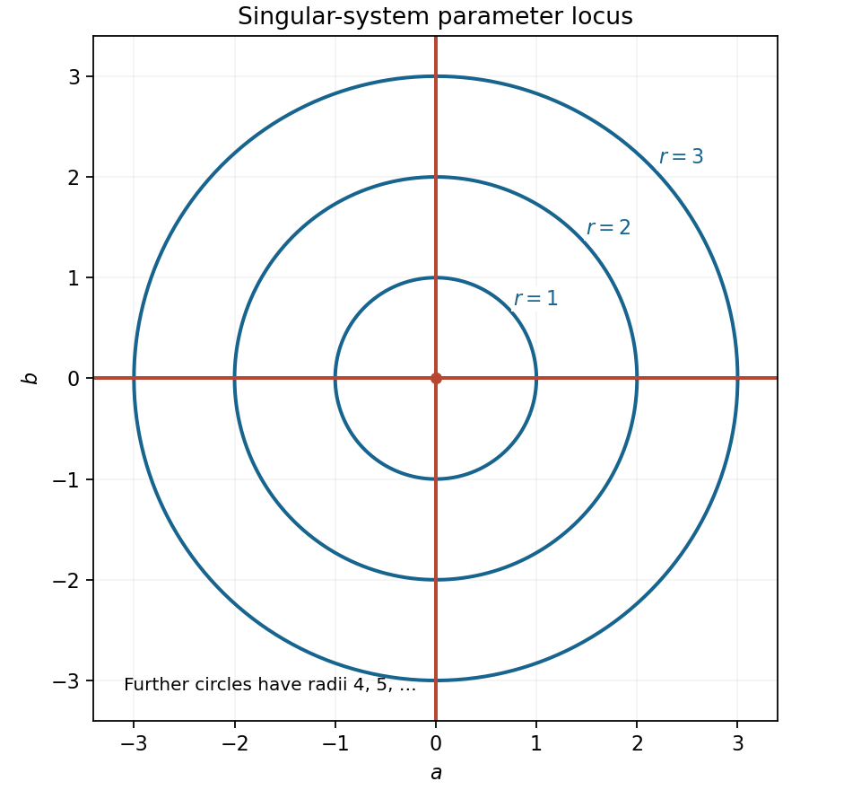
The square roots simplify to the absolute values and . Put . A nontrivial solution of the homogeneous linear system exists exactly when its coefficient matrix is singular:The second factor vanishes precisely when , or , giving both coordinate axes. The first factor vanishes when is a nonnegative integer. Hence the complete locus isThese are the two axes together with concentric circles of positive integer radii. The zero-radius case is the origin, already included on the axes; at that point both equations vanish and any nonzero pair works.
Collect the coefficients of the three unknowns in rows. The linear system has matrix formThe next two parts solve this same system by the two requested methods.
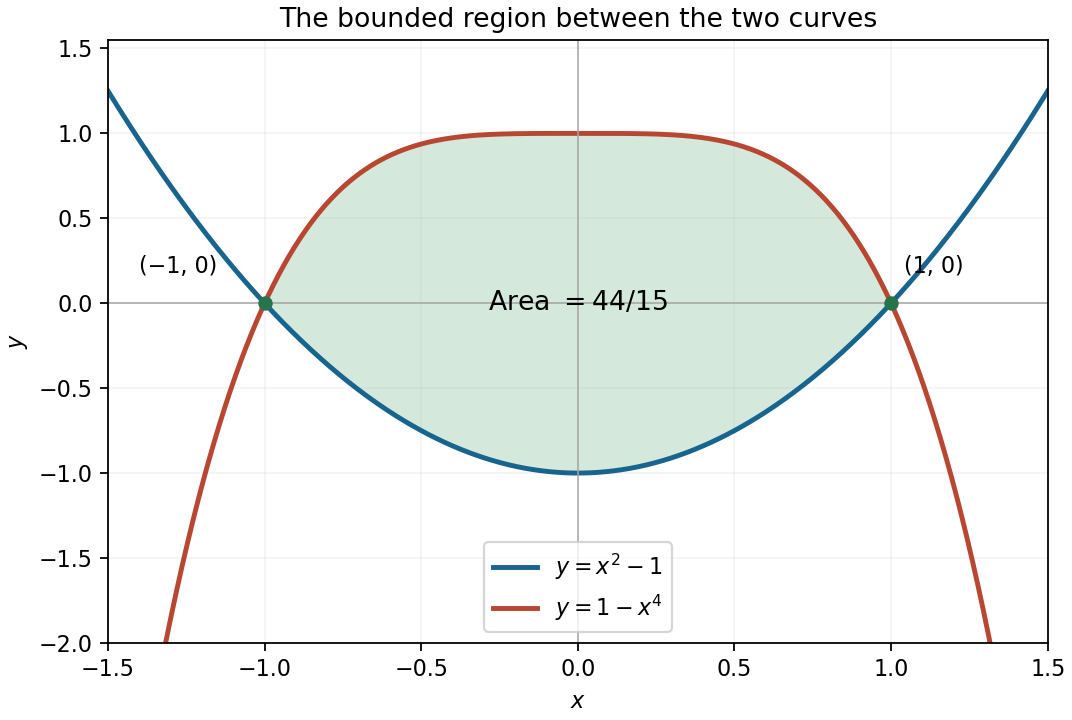
Subtract the lower curve from the upper curve on the intersection interval. The definite integral isThe result is in square coordinate units.
The parabola opens upward, with its minimum at and zeros at . The quartic graph is symmetric about the vertical axis, has its flat maximum at , and also has zeros at .


Use implicit differentiation, treating as a function of :Where , this is . At the two points where , the ellipse has vertical tangent lines rather than a finite slope.
Insert the linear initial profile into the transformed integral from (b):The constant part integrates to . The other part is an absolutely integrable odd function, so its integral vanishes. HenceAs a direct check, and . Thus a linear temperature profile is stationary on the whole line. More generally, every affine function is preserved by this heat-kernel solution.
The indicated integration by substitution givesPointwise, the argument of tends to . Since the Gaussian integral is , the expected limit is . To justify it for unbounded data, use the approximate identity property rather than assuming a uniform bound on .
In the original variable, normalization givesFor , continuity makes the difference smaller than any prescribed if is small enough, and the kernel mass is at most one. On the complement the Gaussian mass tends to zero; the data-weighted tail tends to zero by heat-kernel convergence for Gaussian-integrable initial data. This provesFor heat-kernel convergence from a conditionally convergent Gaussian integral, the same tail conclusion follows using the bounded primitive of . The factor has its maximum at , approaching . For sufficiently small , it is monotone on each of the two tails outside , and its values at the tail endpoints tend to zero exponentially. Integration by parts bounds each tail by a constant times its endpoint value, proving the same limit without an absolute-convergence assumption. The approach is from positive time.
Write the kernel as , with . Its partial derivatives areThus the heat kernel itself satisfies . The proposed convolution consequently givesThis verifies the heat equation. The parameter is positive time; the real integral formula is not defined at negative time.
The passage of derivatives through the integral needs justification. A sufficient condition is the Gaussian-weighted absolute integrability in heat-kernel convergence for Gaussian-integrable initial data; it holds, in particular, for data of polynomial growth. On compact positive-time intervals strictly below an integrable later time, the differentiated kernels have an integrable Gaussian bound, so differentiation under the integral sign applies.
Even if the PDF's assumed convergence is read as ordinary conditional convergence, one can justify the same calculation. Choose a later time and let be a primitive of . Convergence at spatial point zero and time makes bounded on both tails. Put . This function, its spatial and time derivatives, and their -derivatives decay as Gaussians when . Integration by parts rewrites the convolution as , with vanishing endpoint terms. Boundedness of now permits differentiation under this absolutely convergent integral; since , the same equation follows. Thus one need not silently equate conditional and absolute convergence.
For ,In particular its absolute value is bounded by , proving convergence when ; the apparent endpoint singularity at one is removable, with value . On any compact parameter interval with lower bound , the differentiated integrand is , dominated by . The dominated convergence theorem therefore justifies differentiation under the integral sign:Hence . Since the integrand is identically zero at , fixes . ThusThis proves the logarithmic integral representation of the natural logarithm, including its parameter range.
The Leibniz integral rule accounts for both the moving upper endpoint and the integrand's dependence on :For the specified integrand this gives . When , integration by parts givessoFor the requested independent check, direct integration gives at . Its derivative is , agreeing with the result above. At zero the apparent singularity is removable: , so .
Let denote a green pear on the first draw and a red apple on the second. The two categories are disjoint, so after there are still three red apples among seventeen remaining fruits. Thus . Using from (c), conditional probability givesEquivalently, conditioning on the second fruit being one particular category removes a red apple and leaves the other seventeen fruits symmetrically eligible for the first position.
Condition on whether the first selection was a red apple. Its probability is . If it was, two red apples remain among seventeen fruits; otherwise three remain. The law of total probability givesThe same result follows from exchangeability: before either selection is observed, each ordered draw position has the original red-apple fraction , despite dependence between the draws.
Insert the values from (a) into Bayes' theorem:Thus the identity is satisfied. Equivalently, both and equal the joint probability .
There are eighteen equally likely first choices. Counting the relevant subsets givesFor conditional probabilities, restrict the denominator to the conditioning subset:The five counts come from the same finite sample space, so no independence assumption is involved.
There are unlisted articles, also show them or only show them.