
Beyond-all-orders boundary-value sensitivity Created 2026-10-14 Updated 2026-10-25
A homogeneous mode can be order one inside an interval and exponentially small at an endpoint. Adjusting an endpoint value beyond all algebraic orders can then change the interior solution by order one. In the nested layers at an essential singular endpoint example, the mode has this behavior: prescribed exact endpoint values give a unique solution for each fixed positive , but leading asymptotic endpoint data do not select a unique bounded family.
Singular isothermal sphere lens Created 2026-10-14 Updated 2026-11-05
The projected density gives cylindrical mass , so the reduced deflection magnitude is the constant displayed angular Einstein radius. The signed thin gravitational lens equation is . A source with has two images; one with has one. The lensing convergence and lensing shear magnitude are both .
Local coefficient system 2026-10-14
A local coefficient system assigns an Abelian group or module to each point, with compatible transport isomorphisms along paths depending only on homotopy relative endpoints. Equivalently it is a functor from the fundamental groupoid. On a connected manifold it is described by a representation of the fundamental group after fixing one fiber.
Small singular chains for an open cover 2026-10-14
For an open cover, take the subcomplex generated by singular simplices whose images lie in single cover members. Repeated barycentric subdivision makes each finite singular chain small, and the standard subdivision chain homotopy shows that inclusion induces homology isomorphisms. For a two-set cover, the short exact sequence of these small chains gives the Mayer–Vietoris sequence; excising the complement of one open set from the pair with the other set gives its equivalent relative-homology formulation.
Singular chain complex Created 2026-10-14 Updated 2026-10-31
The chain complex whose degree- group is freely generated over by the singular simplices . Its boundary is the alternating sum of restrictions to codimension-one faces. The homology of this complex is singular homology.
Combine the single-copy Werner filtering normalization bound with concurrence scaling under invertible local filters. Every complete classical record of local operations and classical communication has a product filter ; singular branches are separable. Thus every retained branch has concurrence at most that of the input. Coarse-graining successful records preserves the bound by convexity. Since concurrence of a two-qubit Werner state increases strictly with , no successful single-copy protocol can output a Werner state with larger . Several input copies permit collective distillation and are outside this statement.
In dimension three, the first three vertices are . Their closed vertex neighbourhood has seven vertices. Adding does not change that vertex neighbourhood, so the external vertex boundary decreases from four to three even though both family sizes are at most half the cube.
In the seven-dimensional Boolean hypercube, contains every set of size at most three except . Its external vertex boundary consists of that missing triple and all 35 four-sets. The complementary-size initial segment contains every set of size at most three and . Its external vertex boundary has the other 34 four-sets and three five-sets. Thus complementary family sizes do not impose a symmetric boundary profile.
Positive alternating simplex Created 2026-10-14 Updated 2026-10-25
For a simplicial map to the standard simplicial decomposition of a sphere, a -simplex is positive alternating when its image has the displayed distinct labels. Reversing all signs makes it negative alternating. A collapsed or nonalternating simplex is neutral. Counting positive facets modulo two is the local ingredient in the antipodal alternating-simplex parity lemma.
If a variable gains an objective coefficient , the new objective is . Substitute this in the old canonical objective equation and eliminate any remaining basic-column coefficients using the constraint rows. If is nonbasic, this simply subtracts from its objective-row coefficient. When a slack variable is sold, rename the old slack as the sales quantity; its equation already gives the correct equality and no new slack is added. Reoptimization can then start directly from the altered simplex tableau.
For a maximization problem with unpriced unit slack variables, their columns in a final simplex tableau give , where consists of the original basic columns. The constraint right side is , so . If the objective row uses reduced costs , its slack entries are with . Therefore . In a homogeneous linear objective with no constant offset, the displayed basic objective value must equal . This identity detects inconsistent tableau constants; an affine offset affects the value but not the reduced costs.
Basic variable 2026-10-14
A basic variable corresponds to a column of the current simplex basis. Given the nonbasic variables, the invertible basis matrix determines the basic variables from the equality constraints.
// Target: mathematical-optimization.bigb
Nonbasic variable 2026-10-14
A nonbasic variable corresponds to a column outside the current simplex basis. In standard nonnegative linear programming, it is set to zero at the basic solution. With explicit finite bounds, it is normally fixed at one of its bounds.
// Target: mathematical-optimization.bigb
For positive smooth tube area , the equation becomes under the displayed transformation. Indeed, cancels geometrical spreading and makes the remaining nonlinear and transport coefficients equal. Starting with gives and ; characteristic crossing first occurs when , if that supremum is positive.
Sample mean under simple random sampling Created 2026-10-14 Updated 2026-11-05
Fix real population values . Define the finite population mean and two normalizations of the finite population variance byThe values are fixed; only the selected subset is random. For its sample mean , the exact design expectation and variance areThe sample mean is an unbiased estimator of the finite population mean. At , every unit is observed and exactly, so the variance is zero. The case is deterministic and is handled directly, since is undefined then.[ref]
Chapter 2: Simple Random Sampling. Sampling Theory, Chapter 2, PDF pp. 2, 6–9: variance normalizations, unbiasedness, covariance derivation and finite population correction
The finite population correction depends on the baseline. With the normalization it is multiplying . With the normalization it is multiplying , the exact variance for independent uniform sampling with replacement. The standard error uses the square root of the relevant variance factor. Mixing the two normalizations gives a wrong answer even at , when replacement cannot matter. For the six-value example, , , and , reproducing without replacement and with replacement.
A short proof exposes the statistical dependence. Let be the value at position in uniform sequential sampling without replacement, so each has expected value and variance . Write . Every ordered pair of distinct labels is equally likely, and , hence for ,Linearity of expectation proves unbiasedness without requiring independence. The variance of a sum includes all ordered covariance terms, givingFor the original population, each pair of distinct draw positions has covariance . Drawing a high value leaves a lower mean among the remaining values, balancing subsequent draws. Equal marginal probability distributions therefore coexist with negative covariance.
When , the sample variance is an unbiased estimator of . To check this independently, use : its expected value is . Thus unbiasedly estimates the variance of the sample mean; its square root estimates the standard error, but need not be unbiased.[ref]
Chapter 2: Simple Random Sampling. Sampling Theory, Chapter 2, PDF pp. 10–12: sample-variance and standard-error estimation
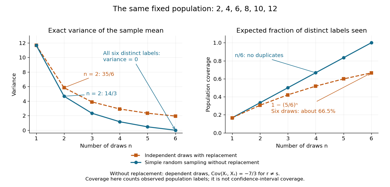
Exact mean variance and expected distinct-unit coverage as sample size grows in the six-value population
. Details. 
The diagram compares variance with the expected fraction of distinct population labels observed. Without replacement this fraction is exactly ; with independent uniform sampling with replacement, a label is missed with probability , so linearity of expectation gives expected fraction . At six draws, replacement covers only about of labels on average and retains sample mean variance ; sampling all six distinct labels covers the population completely and removes selection uncertainty. This population coverage is distinct from confidence interval coverage probability.
The correction matters when the sampling fraction is appreciable. It calibrates uncertainty about this fixed population under the specified selection mechanism. It does not correct unequal selection weights, missing observations or measurement errors; observing every label also does not eliminate uncertainty about a larger unobserved population. Moreover, an exact variance alone does not guarantee the coverage probability of a proposed confidence interval: a small discrete sampling distribution can make a normal approximation inaccurate.
Dyadic occupancy approximation of a simple point measure Created 2026-10-14 Updated 2026-11-05
For a fixed bounded interval with no atoms at its endpoints, the occupation count of fully contained half-open dyadic intervals increases to the true count of a simple locally finite point measure. Refinement cannot reduce occupancy. Finitely many distinct atoms in a bounding interval have positive minimum separation; for fine enough cells each atom lies alone, and every interior atom's cell is contained in the target interval. Thus the counts eventually agree, path by path.
Fixed-endpoint harmonic-oscillator action Created 2026-10-14 Updated 2026-10-18
For and fixed endpoint values , the Euler-Lagrange equation is . When , solve the endpoint equations for the unique trajectory and use on that trajectory to obtain the displayed action. For , at a solution exists only if ; then there is a family of solutions and their action is zero. At the nonresonant formula has the limit .
For a finite simple group of this order, gives a normal Sylow -subgroup, and gives a nontrivial sign homomorphism from the regular action, because an involution swaps fifteen pairs. Thus . The Sylow -count divides ; it cannot be one or three. If it is five, a Sylow subgroup's normalizer has index five. If it is fifteen, the strengthened Sylow congruence from intersections produces two Sylow subgroups meeting in index two. Their common subgroup is normal in both, so its normalizer contains both and has index three or five. Simplicity excludes index three. The resulting faithful degree-five action embeds in and forces order , proving the conclusion.
Finite simple group Created 2026-10-14 Updated 2026-11-05
A nontrivial finite group whose only normal subgroups are the trivial group and the whole group. A cyclic group of prime number order gives an abelian example; gives a nonabelian alternating group example. Finite versions of classical groups can produce further examples after taking suitable subgroups and quotients; small parameters require separate checks.
Viscometric flow Created 2026-10-14 Updated 2026-11-05
A viscometric flow has the local relative deformation history of steady simple shear flow, up to rigid changes of frame. For an isotropic simple fluid, symmetry leaves one shear stress and two independent normal-stress differences. The corresponding viscometric functions depend on the magnitude of the shear rate, while pressure supplies the isotropic part.
There are unlisted articles, also show them or only show them.