
Character space of an Abelian L1 group algebra Created 2026-10-14 Updated 2026-10-31
For a locally compact Hausdorff Abelian group, each continuous unitary character defines an algebra character by . Conversely, if is a nonzero algebra character and , the ratio is independent of , continuous and multiplicative. Translation isometries bound all its integer powers, so its modulus is one. The convolution formula recovers . The Gelfand topology corresponds to the compact-open topology on the Pontryagin dual group; conjugating the characters gives the alternative Fourier sign convention.
Essentially bounded function 2026-10-14
A measurable function is essentially bounded if some finite nonnegative real number bounds its absolute value almost everywhere. The exceptional null set may contain arbitrarily large values. With Lebesgue measure on , a function equal to zero outside and equal to at is essentially bounded despite being unbounded pointwise: its exceptional countable set is a null set, so works. Its L-infinity norm is zero because it represents the zero equivalence class in Lp space.
Contrast this with on . For every , the values exceeding occupy , a set of positive Lebesgue measure. Hence no finite almost everywhere bound works, and this function is not essentially bounded. Being finite at every input does not imply essential boundedness.
Scale-free Kuzmin superposition 2026-10-14
For and , the unreferenced relative potential of the Kuzmin reflection method diverges at large . Referencing each component to the origin before integrating gives the finite potential differenceAt small the subtraction is integrable because ; at large the difference is , integrable because . Its plane force is , where . A circular speed fixes , givingThe beta function substitutions for the force and surface density have different exponents. Its central mass is locally finite, but its total mass diverges at large radius; a potential zero at infinity cannot be imposed. The force and density approach those of the Mestel disk as .
Central contribution to kurtosis 2026-10-14
For a standard score and , split kurtosis into the contribution from within standard deviations of the mean and the contribution from outside:The indicator function selects the central outcomes. The bound follows directly from there. Thus : when kurtosis is large, any fixed central range contributes a small fraction. This is a precise reason to emphasize extreme standard scores rather than peak height.[ref]
Kurtosis as Peakedness, 1905 – 2014. R.I.P. by Peter H. Westfall. §5, Why Tails Mostly Determine Kurtosis, inequality (1) and following fixed-h argument
For the rare-outlier three-point distribution with , and . At the other endpoint , all probability mass lies at , so : central dominance is possible when kurtosis is small. More generally, the Cauchy-Schwarz inequality gives ; the equally weighted outcomes attain this minimum.
Affine invariance of kurtosis 2026-10-14
Changing units or shifting the origin preserves kurtosis. For real constants and , the mean of is , its variance is , and its fourth central moment is . The factors cancel in the ratio, even for negative . Hence excess kurtosis is also unchanged. For example, and have the same kurtosis, although their means and variances differ. The case produces zero variance and is excluded.
Rare-outlier three-point distribution 2026-10-14
For , put probability mass at zero and at each of and . This symmetric probability distribution has mean zero. Its second and fourth moments are both , because the nonzero outcomes have square and fourth power equal to one:For the kurtosis is ; for it is . In the latter case of the probability mass is at zero, yet all of the fourth central moment comes from the remaining . The standard score takes values and , with variance one. Each nonzero outcome contributesto kurtosis. At , the two rare outcomes are ten standard deviations from the mean, and their contributions are .
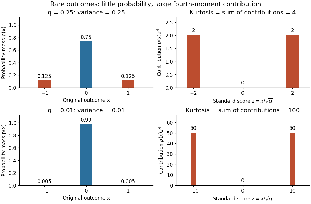

Every member has finite support of a probability distribution, so all its moments are finite. Nevertheless, kurtosis becomes arbitrarily large as approaches zero: high kurtosis does not require an unbounded support of a probability distribution or a heavy-tailed distribution. At the variance vanishes and kurtosis is undefined. At this discrete probability distribution even has the normal distribution value and excess kurtosis zero, so those values do not establish a normal distribution.
Excess kurtosis 2026-10-14
Excess kurtosis subtracts from kurtosis, making the normal distribution baseline zero. The non-excess convention is sometimes called raw kurtosis; this still uses a fourth central moment, not the uncentered fourth moment . Software may report either kurtosis or excess kurtosis, so the convention must be stated.[ref]
1.3.5.11. Measures of Skewness and Kurtosis. §1.3.5.11, Alternative Definition of Kurtosis, normal baseline and software convention warning
For a standard normal distribution, the moment-generating function of a standard normal variable gives , hence excess kurtosis zero. For a continuous uniform distribution on , the mean is zero, the variance is one, and direct integration givesThe rare-outlier three-point distribution can instead have kurtosis and excess kurtosis with mean zero and variance one. These are calculated properties of specified probability distributions, rather than a measured statistic.
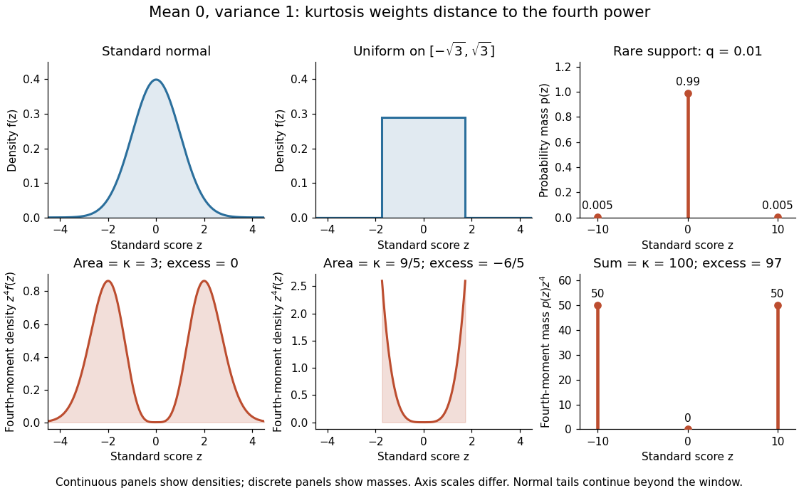
Kurtosis comparison for a standard normal distribution, a continuous uniform distribution, and a rare-outlier three-point distribution
. The upper panels show probability density functions or a probability mass function; the lower panels show their contributions to the fourth central moment. All three probability distributions have mean zero and variance one. Areas in the continuous panels and sums in the discrete panels give kurtosis. The standard normal distribution continues beyond the displayed window; density and mass heights have different meanings. Details.
For finite cell complexes, the cohomological cross product gives a split, but not naturally split, short exact sequence . The Tor degree is for cohomology, unlike the shift in the homological version. If one factor's cohomology is free, the Tor term vanishes and the resulting ring is the graded tensor product.
Cohomological Künneth theorem over a field 2026-10-14
If is a field and has finite total dimension, the cohomology cross product gives the displayed graded-ring isomorphism for arbitrary spaces. Over a field, every chain complex splits into its homology with zero differential and contractible summands. The Eilenberg–Zilber theorem thus replaces the fiber chain complex by a bounded finite-dimensional complex; dualizing its tensor product with gives a finite direct sum of shifted cochain complexes of . Its cohomology is the displayed tensor product. Finiteness prevents the infinite-product obstruction that can occur for two infinite discrete spaces. The standard product formula and its finiteness hypothesis are discussed in pi.math.cornell.edu/~hatcher/AT/ATch3.pdf, Theorem 3.15.
Cohomology cross product 2026-10-14
For classes on and , apply the induced maps on cohomology of the coordinate projections and take their cup product on . The result has degree . On a tensor product of graded rings, the sign rule makes this a ring homomorphism.
For an odd prime , the unique quadratic subfield of a prime cyclotomic field has no finite ramification outside . The classification of quadratic discriminants identifies it with , where . A fundamental discriminant factors as with . The remaining quadratic number field is generated by , , or and lies in . Taking the corresponding compositum proves the indicated quadratic case of the Kronecker–Weber theorem.
Closest-root descent in a Galois extension Created 2026-10-14 Updated 2026-11-05
Let be a finite Galois extension of a field complete for a Non-Archimedean absolute value. Let . Suppose is uniquely closest to among the roots of a polynomial over lying in . Every element of preserves absolute values on a field and permutes these roots. It sends to an equally close root, hence fixes . The Fundamental theorem of Galois theory gives . The converse inclusion need not hold: for roots , the element is uniquely closest to zero but does not belong to .
For and normalized at infinity, the Komar mass on a round sphere is . The future unit normal to a static slice is , and the outward unit radial normal is ; their contraction with gives , whose integral over the sphere yields the formula. The asymptotic mass is its limit at infinity. In the presence of matter, the finite-radius integral need not be constant.
For future static-slice normal and outward radial normal , take , with both antisymmetric components summed. For the Schwarzschild-Tangherlini metric the flux is . The displayed dimension-dependent coefficient then reproduces the ADM mass. Reversing orientation reverses the flux; including a factor of one-half in the binormal convention also changes its numerical value. A four-dimensional normalization cannot be carried unchanged into other dimensions.
For an axial Killing vector and zero cosmological constant, set . The Killing equation and Ricci identity give . In a vacuum region this vanishes, so Stokes theorem makes the Komar angular momentum equal on homologous enclosing surfaces. The region may contain gravitational waves with nonzero Weyl curvature: Ricci flatness, rather than complete flatness, is what removes the flux. This proves absence of axial angular-momentum transport by exactly axisymmetric gravitational radiation, without assuming that a radiating spacetime is stationary.
Lognormal intermittency model 2026-10-14
If is Gaussian with variance , normalization gives . Taking predicts . Its eventual negative high-order exponents show that this extrapolation cannot hold for arbitrarily large orders with finite uniform velocity moments.
Kolmogorov first similarity hypothesis 2026-10-14
In the locally isotropic equilibrium range, the small-scale velocity increment statistics depend on the separation, mean viscous dissipation and kinematic viscosity, independently of large-scale forcing details. Dimensional analysis leaves the Kolmogorov microscales as normalization scales and gives the displayed second-order longitudinal structure function. Universality of is part of the hypothesis, not something proved by dimensional analysis.
Kolmogorov second similarity hypothesis 2026-10-14
In the inertial range, velocity increment statistics also become independent of kinematic viscosity. Combined with the Kolmogorov first similarity hypothesis, this gives by dimensional analysis. Signed integer moments and absolute noninteger moments must be distinguished; the signed third-order coefficient is negative in a forward energy cascade.
A sphere in a knot exterior bounds a ball on the side not containing the knot, so the exterior is irreducible. A compression disk for its boundary torus would cut the exterior to a manifold with sphere boundary; irreducibility makes that manifold a ball, and reversing the compression gives a solid torus exterior. Its meridian disk has boundary a preferred knot longitude, so adjoining the boundary annulus gives a spanning disk for the knot, which is then an unknot. The Loop theorem therefore makes the peripheral fundamental group injective for every nontrivial knot. In particular its knot group contains an injected copy of the torus group and cannot be cyclic.
Tait conjectures 2026-10-14
The Tait conjectures concern reduced alternating knot diagrams: they minimize the crossing number of a knot, have an invariant diagram writhe, and are related by flypes. These formerly conjectural assertions are now theorems; the first is the Tait crossing-number theorem.
There are unlisted articles, also show them or only show them.