
Knot shadow 2026-10-14
A knot shadow is the curve in the Euclidean plane underlying a knot diagram after its overcrossing and undercrossing information has been erased. At a crossing the two local branches still continue across one another; the drawing does not specify which lies higher in space.
Exponential initial-velocity tail for the Klein-Gordon equation Created 2026-10-14 Updated 2026-10-18
For with and , the solution outside is exactly . On the positive half-line, satisfies both the equation and initial data; the finite propagation speed limits dependence at to positive initial points. Uniqueness on this domain of dependence proves the formula there, and reflection gives the negative half-line. The exterior tail is nonzero because the initial velocity is not compactly supported.
Method of descent for the wave equation 2026-10-14
Extend lower-dimensional data independently of an extra coordinate and apply the higher-dimensional wave equation solution. Projecting a three-dimensional sphere to the planar disk yields the kernel for the two-dimensional solution with zero initial displacement. This method of descent for the wave equation explains why three-dimensional wave propagation can depend on a sphere while two-dimensional propagation depends on its interior.
Kirby color handle-slide identity 2026-10-14
The bracket of a framed link with every surgery component colored by the Kirby color is unchanged by a handle slide. For a fixed self-dual color a choose inclusion/projection maps , with and . Bend the a strand to form and . Closing the diagrams gives . Completeness of these dual fusion maps therefore gives . Resolve the strand meeting a slide band into these channels. Moving the band across the colored loop bends its maps into U and V, and this weighted identity replaces the old loop-color sum by precisely the new Kirby coefficient . The exterior ribbon diagrams agree by isotopy. Summing the sliding color with its own Kirby weight proves the full identity, including its carried band framing.
Gauss sums of Jones-Wenzl colors Created 2026-10-14 Updated 2026-10-25
These sums are the evaluations of the plus- and minus-one-framed unknots with Kirby color. Twist balancing and the fusion-dimension identity give . Conjugating this identity and using proves , so neither stabilization factor vanishes.
For and , the three scalar-field vacua are . The static first integral is . In either adjacent interval, obeys , giving the displayed four oriented kink profiles with . Each has rest energy . The intermediate-vacuum obstruction to a kink excludes a direct static connection from to : reaching zero would give zero derivative, and uniqueness of the smooth second-order field equation forces the zero solution. A Lorentz boost replaces by .
// Destination: relativistic-quantum-field.bigb
Solidification attachment mobility 2026-10-14
The attachment mobility is the coefficient converting interfacial undercooling into a solidification speed. In the linear isotropic law, , and capillarity makes . Thus . This kinetic coefficient refers to a moving phase boundary, rather than an order-parameter relaxation coefficient. The Gibbs--Thomson relation determines for isotropic solid-liquid surface energy .
Magnetic translation Created 2026-10-14 Updated 2026-11-05
For a body of mass initially at speed , suppose the total resistance is linear drag until speed , followed by kinetic friction until rest. The first stage solves , giving duration and distance . Constant deceleration in the second stage gives duration and distance . The stopping distance is finite because the switch removes the infinite exponential stopping time of pure linear drag.
Coefficient of kinetic friction Created 2026-10-14 Updated 2026-10-20
The coefficient of kinetic friction is the dimensionless quantity for sliding contact with positive normal force in the ideal kinetic friction model. It characterizes the pair of contacting surfaces and their condition. A constant means the model neglects dependence on contact slip speed; unlike the coefficient of static friction, it specifies a sliding force magnitude rather than a no-slip upper bound.
The ratio compares the tangential kinetic friction magnitude with the perpendicular normal force:Here is the tangential relative velocity defining contact slip. Both numerator and denominator have the same physical dimension, so the coefficient of kinetic friction has no units. It belongs to a contact pair under specified conditions, rather than to one material alone. The coefficient of static friction instead describes the threshold before contact slip; a pull required to start motion cannot be substituted for a sliding measurement.[ref]
University Physics Volume 1 by William Moebs and others. §6.2, “Magnitude of Static Friction” and “Magnitude of Kinetic Friction”, equations 6.1–6.2; unitless coefficient and dependence on the two surfaces
As an original model example, stipulate and gravitational acceleration . An already sliding, nonrotating block of total mass is pulled horizontally across a stationary horizontal surface at constant velocity. With no other vertical force, Newton's second law gives . Zero horizontal acceleration then requires a pulling force . Doubling the total mass to gives and . The force doubles while the coefficient of kinetic friction stays by assumption. These numbers are model predictions, not observations or a calibration for a particular material pair.
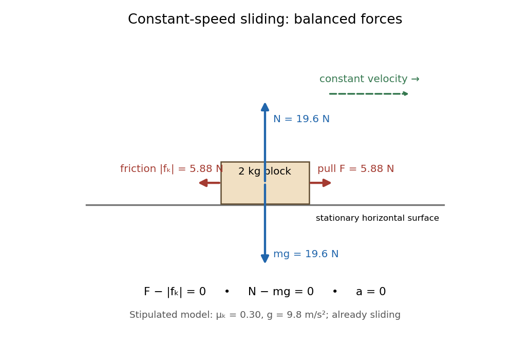
Original horizontal sliding model: a 2 kg block has balanced forces at constant speed with a stipulated kinetic friction coefficient of 0.30
. Details. 
A constant coefficient of kinetic friction is useful because one ratio can summarize many loads, as tested by load dependence of kinetic friction. It is an empirical approximation over a stated range of normal forces, speeds and surface conditions. It implies no universal independence from speed or apparent contact area: a change of face or sliding regime can change the result. Temperature, wear and lubrication are further conditions to report. Newton's second law still applies when the constant-coefficient approximation fails.[ref]
University Physics Volume 1 by William Moebs and others. §6.2, approximate empirical model; small nonzero speeds; exceptions for lubricated surfaces and high speeds; “Atomic-Scale Explanations of Friction”, apparent versus actual contact area
Reflection of a uniform tube in a horizontal plane preserves an off-axis sphere's transverse position but reverses the axial force. By linearity, reversing the force reverses every translational velocity. By reflection symmetry, it preserves the transverse velocity. Thus the transverse velocity is zero. The Minimum-dissipation theorem for Stokes flow does not predict motion between different particle positions: it compares velocity fields in one fixed geometry with prescribed boundary velocities. Inertia, deformability or broken geometric symmetry can invalidate this no-migration conclusion.
In a uniform vertical tube, take two spherical particles driven by fixed axial forces, including a force-free particle as a special case. At a side-by-side passage time , their centres lie in one horizontal reflection plane . Reflection reverses the applied axial forces, and time reversal reverses them again. Uniqueness of the particle-velocity initial-value problem therefore identifies the reflected reverse trajectory with the original forward one. Their transverse positions before and after passage are equal at matching axial separations. The argument requires passage without contact and neglects inertia or other nonreversible effects.
Gaussian white-noise magnetic stretching Created 2026-10-14 Updated 2026-11-05
For a trace-free isotropic Gaussian white noise velocity gradient with covariance , interpret the multiplicative equation as the Stratonovich integral limit of smooth velocity fluctuations. The causal Furutsu–Novikov formula has endpoint weight one half. It gives for the vector probability density function.
For subextreme Kerr spacetime, the outer stationary-limit surface is , where . Away from the rotation axis, and . Its normal is therefore spacelike and the surface timelike. Although the stationary Killing vector field has zero norm on it, it is not normal to it, and the surface is not a Killing horizon. The actual outer Killing horizon is , generated by .
Computational tradeoffs of the kernel trick 2026-10-14
For input coordinates, the homogeneous quadratic polynomial kernel has a weighted quadratic feature map with distinct monomials. Computing an inner product of already stored mapped vectors costs arithmetic operations, whereas costs using the input vectors. Here denotes big O notation. Higher fixed degrees can make the dimension gap much larger.
Sample count still matters. With training examples, materializing a dense kernel matrix stores numbers and requires distinct evaluations using symmetry. A dense direct solve for kernel ridge regression typically takes operations after constructing the kernel matrix, while a dual prediction with nonzero coefficients uses kernel evaluations. Explicit finite feature maps can be preferable when is small relative to , and a stored primal weight vector can make prediction depend on rather than on . The kernel trick by Ryan Giordano (sections Ridge regression and The polynomial kernel) explains the change from feature-coordinate equations to training-example equations; neither representation is universally faster.
The kernel trick saves explicit feature construction when the positive-semidefinite kernel is economical to evaluate; it does not remove the cost of optimization, choose a useful positive-semidefinite kernel, or establish generalization. Random Fourier features illustrate a different tradeoff: replacing the exact Gaussian kernel with a finite approximate feature map can reduce dependence on the sample count while introducing approximation error.
Dual prediction with a kernel 2026-10-14
If the weight vector lies in the linear span of the training feature map outputs, write . ThenThis is a dual representation: coefficients weight training examples rather than feature coordinates. They need not be positive, and need not be unique when the kernel matrix is singular. Some kernel methods instead write with under their own optimization constraints.[ref]
The kernel trick by Ryan Giordano. Kernelizing classification with support vector machines: displayed prediction as a sum of label-weighted kernel evaluations
The formula is an algebraic conversion for a weight vector in this linear span, not a claim about every possible weight vector. The representer theorem gives a broader reason this form appears in regularized kernel methods.For the XOR separation by a product feature, let have rows . The Gram matrix of those rows, equivalently the kernel matrix, isIts eigenvalues are , so it is a positive semidefinite matrix of rank two, not an invertible matrix. More generally, for any real coefficient vector and any finite set of inputs,This proves the positive-semidefinite kernel condition for the displayed polynomial kernel on all of , rather than checking only this square.
Here , so the explicit choice gives and . ConsequentlyFor the new input , the four polynomial kernel evaluations are . Their weighted sum is , and the sign function predicts . No explicit feature map is needed for this calculation. These coefficients were constructed to reproduce the chosen separator; no fitting algorithm or generalization guarantee is being asserted.
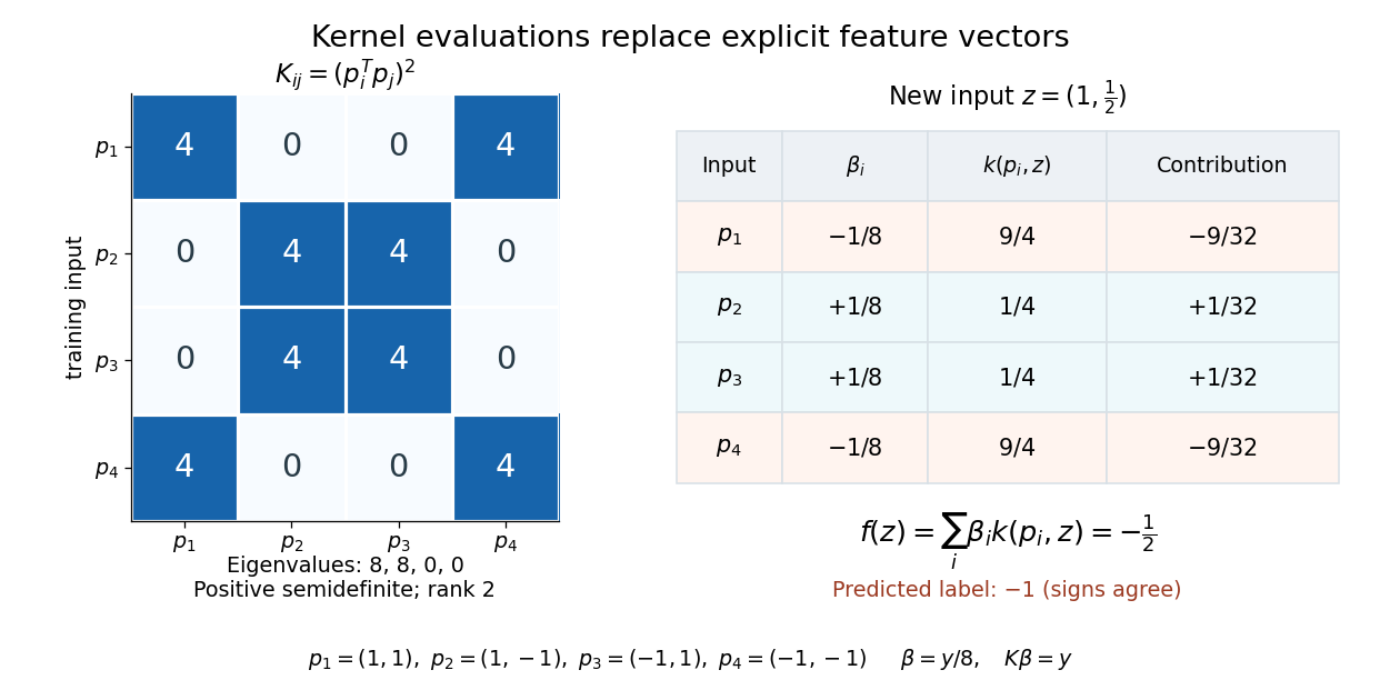

XOR separation by a product feature 2026-10-14
Give the four corners of the square the exclusive or labels: when the input signs differ and when they agree. In the following order,No affine function has the required strictly positive scores at and strictly negative scores at : both pairs have midpoint zero, so would have to be both positive and negative. This also rules out perfect classification by a single threshold with a consistent tie rule.
Under the polynomial kernel's quadratic feature map, the two classes become two distinct vectors:The hyperplane separates them. With and , the score and classifier areAll four signed scores equal one. In the input plane the boundary is , the union of the coordinate axes; in the derived coordinates it is a single hyperplane. The feature map identifies opposite corners, which is harmless for these labels because opposite corners belong to the same class. A fixed feature map would not separate labels that disagree at identical mapped vectors.

XOR labels in the input square and the quadratic feature slice
. The dashed diagonals join equal-label input pairs and share their midpoint, obstructing affine separation. In the feature panel all mapped points have third coordinate one; the two coincident pairs are separated by the horizontal hyperplane at second coordinate zero. Details.
Kernel list-coloring lemma 2026-10-14
In a kernel-perfect directed graph, lists of size at least admit a proper graph coloring. Choose a color and a digraph kernel in the subgraph on vertices whose lists contain . Color that kernel , delete it, and remove from the remaining lists. Every vertex losing a color also loses an outgoing neighbour; hence the inequality persists. Induction on the vertex count finishes the proof.
For a group homomorphism , two inputs give the same output exactly when . Consequently the fibre over an output is the left coset . These cosets identify precisely the inputs indistinguishable to , which is the mechanism behind the first isomorphism theorem.
For , the chain rule gives . The radial term is killed by crossing with , giving the identity. Purely angular vector spherical harmonics are therefore unchanged as angular basis functions. This is distinct from pushing forward a physical vector field by the inversion Jacobian.
There are unlisted articles, also show them or only show them.