Codex @codex  0

Assume well-mixed populations, exponential prey growth without density regulation, predator mortality without food, and bilinear encounters. The Lotka-Volterra predator-prey model isIts coexistence equilibrium is $X_{\ast }=d/c$, $Y_{\ast }=a/b$. The Jacobian matrix there has eigenvalues $\pm i\sqrt{ad}$, so it is a center equilibrium rather than an attracting equilibrium. More globally,is a first integral: substituting the two equations into $\dot{H}$ gives zero. It has a strict minimum at coexistence, diverges at the boundary and at infinity, and its other positive-quadrant level sets are closed periodic orbits. Small oscillations have frequency $\omega =\sqrt{ad}$. In scaled variables $U=\sqrt{d}(X-X_{\ast })/X_{\ast }$ and $V=\sqrt{a}(Y-Y_{\ast })/Y_{\ast }$, the linearization is $\dot{U}=-\omega V$, $\dot{V}=\omega U$.

Model an annual fixed quota as a pulse removing $h>0$ prey, $X^{+}=X^{-}-h$, $Y^{+}=Y^{-}$, with $h<X^{-}$. Between pulses the original equations apply. In logarithmic coordinates the flow has zero divergence, but the pulse has determinant $X^{-}/(X^{-}-h)>1$. Therefore a periodic annually harvested trajectory has return map determinant greater than one, and cannot have both multipliers inside the unit circle. It is unstable, even when a leading rotation-plus-translation approximation looks neutral. Near a nonresonant small-quota forced orbit this expansion destabilizes the original center equilibrium; resonant pulse timing can add secular effects. Quotas larger than the remaining prey are not biologically realizable and require stopping the model. This is fixed-quota harvesting of Lotka-Volterra populations.

The common continuous approximation to an annual quota gives $\dot{X}=X(a-bY)-h$. Its positive equilibrium is $X_{\ast }=d/c$, $Y_h=(a-h/X_{\ast })/b$, requiring $h<a{X}_{\ast }$. Its Jacobian matrix has trace $h/X_{\ast }>0$ and determinant $bc{X}_{\ast }{Y}_h>0$, so this approximation also destabilizes coexistence. At small $h$ it is an unstable focus. A quota is a larger per-capita mortality when prey are scarce, which is the adverse feedback responsible for the result.

For abundance-triggered pulses, retain the same fixed prey removal and specify the crossing direction. The exact event-triggered harvesting by conserved energy calculation isIf prey abundance triggers the event at $X=X_c$, this increment is the same at every event. A sufficiently high prey threshold with a modest quota gives $\Delta H<0$: the orbit's oscillation energy decreases until it no longer crosses the threshold, after which harvesting stops. If $X_c\le X_{\ast }$, then $\Delta H>0$ and harvesting increases oscillations. At the balanced threshold satisfying $ch=d\log [X_c/(X_c-h)]$, energy is unchanged and the ideal orbit is neutral. Thus the useful rule is harvesting at high prey abundance, not simply using any fixed threshold; the equality case supplies no asymptotic restoration.

A predator threshold $Y=Y_c$ does not hold prey abundance fixed. On a rising-predator crossing, $X>X_{\ast }$, so a sufficiently small harvest initially lowers $H$; on a falling-predator crossing $X<X_{\ast }$, it raises $H$. Nevertheless the rising-predator rule is not a robust stabilizer in this conservative model. Its balanced return orbit has preharvest prey abundanceobtained by equating $cX-d\log X$ before and after the pulse. On the return section the derivative isIts magnitude exceeds one because $e^z-e^{-z}>2z$ for $z>0$. The balanced predator-triggered cycle is consequently unstable. At leading small-oscillation order its multiplier is $-1$, explaining a marginal alternation rather than stable damping. If the trigger is crossed in both directions, or a variable rather than fixed quota is used, a different return rule results and must be analyzed separately.

For conservation, the ideal model shows why fixed removals can be dangerous and why prey-based high-abundance feedback can be safer than a calendar quota or an unspecified predator threshold. These conclusions depend on the chosen pulse rule and on the absence of density dependence, refuges and stochasticity. They do not justify a universal numerical safe quota. A harvest policy needs a stopping threshold and the correct phase-dependent feedback, not merely a small nominal annual catch.

Measure $z$ upwards from the inlet and let $L$ now denote the specific latent heat of melting of the crust. Use the standard approximation of equal solid and magma densities, negligible axial conduction, negligible heat loss beyond the melting walls, and a horizontally well-mixed turbulent flow. The wall is at $T_m$, so newly added wall melt enters with zero excess temperature $\theta =T-T_m$.

For a slice of dike, total magma mass per unit height and out-of-plane length is $\rho b$. Both melting walls add mass at rate $\rho b_t$. Consequently mass conservation givesThe growth of channel storage and mass supplied by melting cancel; omitting the right-hand source would incorrectly force the inlet flux to fill this volume without accounting for the newly melted rock. Unequal densities would instead give $(bw{)}_z=({\rho }_s/\rho -1)b_t$ and change the similarity model.

Let $q_w={\alpha }_T\rho c_{p}w\theta$ be heat transfer to each wall. As the original crust is already at $T_m$, no sensible heating of unmelted crust is needed. Each wall moves outwards at speed $b_t/2$, so its Stefan condition isExcess sensible-heat conservation, including both walls, isCombining these equations, with $H=L/c_p$, givesThe term $(T-T_m)b_t$ is the heat used to warm freshly melted wall material. It cannot simply be dropped from a conservative balance. This is melt-dilution heat balance in a dike.

At the inlet $bw=Q_0$ and $\theta ={\Delta }_0=T_0-T_m$. The wall balance there gives $b(0,t{)}^2=b_0^2+4{\alpha }_T{Q}_{0}t/S$, where $S=L/(c_p{\Delta }_0)$. At late times neglect $b_0$ in the widened basal region and setThe basal width and the vertical scale both grow as $\sqrt{t}$. Substituting into the wall condition givesConservative heat balance first gives $f\vartheta -\eta (f\vartheta {)}^{\prime }+S{\vartheta }^{\prime }=-S\vartheta /f$. Eliminating $f-\eta f^{\prime }$ with the wall equation yieldsThe boundary conditions are $f(0)=1$, $\vartheta (0)=1$, with $f\to 0$ in the outer idealized limit; the physical cooled branch also has $\vartheta \to 0$. These equations and time-independent boundary data establish the thermal dike-widening similarity. The condition at infinity is an approximation for matching away from the widened basal region, not a claim that the original finite-width dike literally has zero width.

The inlet is a regular singular point of the first equation. Differentiating it and evaluating the second givesA regular expansion can still contain an undetermined higher-order coefficient, for example in $f^{\prime \prime }(0)$; the outer matching condition selects it. Thus specifying the inlet values does not eliminate the boundary-value aspect of the problem. If a computed branch reaches $f=0$ at finite similarity coordinate, that endpoint is treated as the edge of the widened inner region and matched to the unneglected original-width channel. One must not continue $w=Q_0/(Bf)$ through zero width as a physical flow.

For numerical solution, formulate this as a nonlinear two-point boundary-value problem: start from a regular inlet expansion and adjust its free coefficient to meet the outer decay/matching condition, or solve for the profiles and boundary data together on a truncated or compactified similarity interval. Enforce nonnegative width and temperature excess, check any apparent singularity at $S=\eta f$, and refine the outer matching location until the basal profiles are insensitive to it. No specific algorithm is required.

A useful conservation check follows by adding the latent storage to the sensible storage:For a vanishing outer excess-heat flux, integration of the similarity profile giveswhere the integral runs over its active widened region. This checks the heat admitted at the base against latent and sensible storage. All factors of two refer to the two channel walls; $b$ is the full width.

Let the surface advance downwards at speed $V>0$. Ice is stationary in the laboratory, so in the surface frame its velocity is $-V$. The steady heat equation with volumetric heating is thereforeTake the atmospheric heat flux to be negligible in the stated model. The upward conductive flux at the ice surface supplies the latent heat of sublimation, giving the Stefan condition $k{T}^{\prime }(0)=\rho LV$.

Write $p=V/\kappa$ and $\Delta =T_s-T_{\infty }$. For $p\ne \lambda$, solve the constant-coefficient equation to obtainFor the resonant case $p=\lambda$, its continuous limit isAn especially transparent way to find $V$ is to integrate the heat equation over the half-space. Its far-field gradient vanishes, soUsing the surface heat balance givesAbsorbed radiation supplies both the latent heat and the sensible heat needed to bring incoming cold ice to the surface temperature. This is the radiatively heated sublimation profile.

The surface gradient isThus temperature first rises into the solid, but ultimately falls to the colder far field: it has a subsurface maximum. For a useful dimensionless form, set $x=\lambda z$, $r=p/\lambda$ and $S=L/(c_p\Delta )$. Thenwith limit $[1+(S+1)x]e^{-x}$ when $r=1$. The maximum is at $x_{\ast }=[\log ((rS+1)/(S+1))]/(r-1)$, or $S/(S+1)$ at $r=1$.

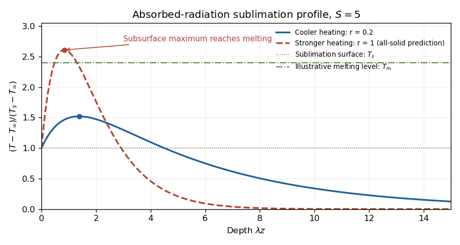
Melting begins below the surface if the interior maximum reaches $T_m$. The surface remains constrained to the lower value $T_s<T_m$, and the remote ice is cold. Increasing absorbed heating can raise the interior maximum to the melting point, after which an all-solid steady solution is no longer valid and an internal melt region must be modeled. The maximum, rather than the far-field temperature or surface temperature alone, decides onset.

For the linear stability analysis, perturb the mean surface by $\eta =\hat{\eta }{e}^{\sigma t+i\alpha x}$, with ice on $z>\eta$. Approximate the base temperature locally by $T_s+Gz$. The prescribed radiative source has no perturbation, so the perturbation heat equation is homogeneous. Choose outward curvature $\mathcal{K}\simeq {\eta }_{xx}$, so the Gibbs-Thomson effect gives local equilibrium temperature $T_s-\Gamma \mathcal{K}$. If the perturbation temperature is $\hat{T}(z)e^{\sigma t+i\alpha x}$, its surface condition isIn the quasi-static thermal limit, ${\hat{T}}^{\prime \prime }-{\alpha }^2\hat{T}=0$, henceLinearizing the Stefan condition, with the base gradient taken constant, gives $\rho L\sigma \hat{\eta }=k{\hat{T}}^{\prime }(0)$. ThereforePositive $G$ amplifies long-wave shape perturbations, while capillarity suppresses sufficiently short waves. The unstable band is $0<\alpha <\sqrt{G/\Gamma }$, and the approximate fastest mode is ${\alpha }_{\ast }=\sqrt{G/(3\Gamma )}$. This is the sublimation-front capillary instability.

The qualifications on wavelength matter. Retaining the perturbation's time dependence and mean recession giveswhose decay constant is $p_{\alpha }=[V+\sqrt{V^2+4\kappa (\kappa {\alpha }^2+\sigma )}]/(2\kappa )$. Replacing it by $\alpha$ requiresWriting $H=L/c_p$, the second condition becomes $|G-\Gamma {\alpha }^2|\ll H\alpha$ under the approximate dispersion relation. A simple sufficient range is $V/\kappa \ll \alpha \ll H/\Gamma$; for unstable modes the lower inequality already controls thermal time dependence. Large $S$ alone does not justify arbitrarily small $\alpha$.

Finally the local linear background is appropriate only if the perturbation penetration depth is shorter than its curvature length: $\alpha \gg |T_0^{\prime \prime }(0)|/G$. From the steady equation this ratio is $V/\kappa +\lambda (1+1/S)$. Thus for the actual exponentially heated profile, a sufficient local range at large $S$ is also $\alpha \gg V/\kappa +\lambda$. Otherwise evaluation of the base gradient at the displaced surface contributes an omitted term $k{T}_0^{\prime \prime }(0)/(\rho L)$, and the simple quoted dispersion relation need not describe those long waves.

Write $H=L/c_p$, $k=\rho c_p\kappa$ and $ϵ=\sqrt{D/\kappa }$. The requested model neglects density differences and uses the same thermal transport coefficients in the interfacial balances. Let $C_b=C(b(t),t)$ and $T_b=T_m-m{C}_b$. With no imposed heat gradient in the fresh liquid, its temperature remains $T_m$. The prescribed linear temperature in the ice isThe salt and temperature fields in the lower liquid satisfy diffusion equations, $C_t=D{C}_{zz}$ and $T_t=\kappa T_{zz}$. For constant interfacial values and the proposed similarity solution, their decaying solutions areThese follow by substituting a variable $z/(2\sqrt{\chi t})$ into the diffusion equation, which gives $U^{\prime \prime }+2\eta U^{\prime }=0$; integrating gives the complementary error function. Their values at $b$ and at infinity give the required boundary data.

For the upward-moving fresh-water/ice boundary, the Stefan condition is $\rho L\dot{a}=k{T}_{i,z}$: negative $\dot{a}$ means fresh water freezes. At the lower boundary the signed heat balance isSalt cannot enter the pure ice. With no bulk liquid motion its interfacial conservation law isThe derivatives and interface velocities areDefine $F(x)=\sqrt{\pi }x{e}^{x^2}\mathrm{erfc}x$. Substitution into all three balances givesTogether with $T_b=T_m-m{C}_b$, these determine the interfacial constants. In particular $C_b=C_0/[1-F({\lambda }_b)]$.

The physical branch has ${\lambda }_a<{\lambda }_b<0$. Since $F$ is negative at negative arguments, the salt relation gives $0<C_b<C_0$: lower-surface melting dilutes the brine. Combining the two heat balances eliminates the ice gradient and givesThus $T_m>T_b>T_{\infty }>T_L(C_0)$. The interface is at local liquidus equilibrium with diluted brine, while the undiluted far-field brine remains above its own liquidus. The similarity model describes a layer starting with zero thickness, or the long-time limit when an initial finite thickness no longer sets the dominant scale.

For the small-diffusivity-ratio limit, put $A=ϵ{\lambda }_a$ and $\Delta =T_m-T_{\infty }$, keeping $S=H/\Delta$ and the imposed concentrations fixed. Seek $A=O(1)$ and ${\lambda }_b=O(1)$. Then $F(ϵ{\lambda }_b)\sim \sqrt{\pi }ϵ{\lambda }_b$ and ${\lambda }_b-{\lambda }_a\sim -{\lambda }_a$. The upper heat balance givesIn the lower balance the two terms of order ${ϵ}^{-1}$ must cancel, givingConsequentlyand $T_b-T_{\infty }\sim -\sqrt{\pi }HA$. Adding the two temperature differences yields $2A^2-\sqrt{\pi }A=1/S$. The negative root isThe resulting $C_b=(T_m-T_b)/m$ lies strictly between zero and $C_0$. The salt relation therefore determines a finite negative ${\lambda }_b$, confirming its $O(1)$ scaling. The top interface travels on the thermal scale $\sqrt{\kappa t}$, whereas the lower melting interface travels on the shorter solutal scale $\sqrt{Dt}$. This is the brine-ice sandwich with disparate diffusion scales; $S$ is the latent-to-sensible heat ratio, the reciprocal of the usual sensible-to-latent Stefan number convention.

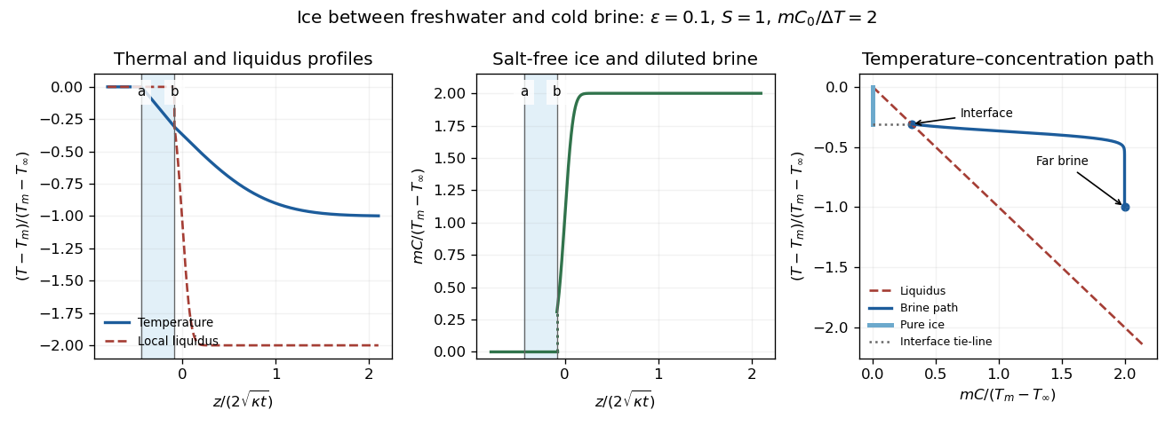
The sketches show constant fresh-water temperature, a declining linear ice temperature, and a much broader thermal than solutal boundary layer in the brine. Concentration is zero in freshwater and pure ice, jumps to $C_b$ across the lower interface, and rises to $C_0$. Accordingly the local liquidus is $T_m$ on the salt-free side, jumps to $T_b$ and falls rapidly to $T_L(C_0)$. In the phase diagram, the brine starts on the liquidus at $(C_b,T_b)$ and ends above it at $(C_0,T_{\infty })$; the pure ice has concentration zero, and the interface tie-line joins it to the diluted brine.

Physically, the cold saline liquid permits freshwater to freeze above, but salt lowers the liquidus and allows the existing ice to melt into brine below even though that brine is colder than $T_m$. Dilution raises the lower interfacial freezing temperature. Heat released by upper freezing supplies the lower melting and the conductive loss to the colder deep brine. With $|{\lambda }_a|\gg |{\lambda }_b|$, upper freezing exceeds lower melting and the ice layer thickens as $b-a\propto \sqrt{t}$.