
Past exam of the mathematics course of the University of Cambridge 2002 iii Paper 63 4 Solution Created 2026-10-03 Updated 2026-10-14
The Adjoint representation of a Lie algebra acts on the algebra itself: . In the basis , its matrices areFor any algebra element , the Jacobi identity givesTherefore the matrices satisfy the same Lie bracket relations:This construction does not require that the algebra be simple or that the adjoint action be faithful.
For the field calculation, write and . In the derivative-plus-connection convention the Yang-Mills field strength isThe sign of the parameter here is the negative of the matter-field parameter in the usual gauge transformation in the derivative-plus-connection convention. Work with the stated throughout. Expanding the variation givesThe second derivatives cancel by commutativity of partial derivatives, and all remaining derivatives of cancel by antisymmetry of the Lie bracket. The Jacobi identity makes the last two terms . HenceUnlike the connection, the curvature has no inhomogeneous derivative term: it transforms in the Adjoint representation.
The quadratic form is the Killing form. Its symmetry follows from cyclicity of the matrix trace. Using the just-proved adjoint commutators,ThusEquivalently, each adjoint generator is skew with respect to this invariant bilinear form. This invariance holds even when the Killing form is degenerate; no inverse form is needed here.
The spacetime metric used to raise Lorentz indices is unaffected by the internal gauge transformation. Since , invariance givesTherefore the Killing-form contraction of the field strengths is gauge invariant, as required for the internal contraction in a Yang-Mills action.
Past exam of the mathematics course of the University of Cambridge 2002 iii Paper 63 3 Solution Created 2026-10-03 Updated 2026-10-14
For a Cartan-Weyl basis, the Jacobi identity givesThus the bracket has joint Cartan weight . If , it belongs to the zero-weight space, which is the Cartan subalgebra, and so is a linear combination . If is a nonzero root, its root space is one-dimensional and the bracket is proportional to . If that nonzero sum is not a root, the bracket vanishes. This proves the asserted forms without assuming every pair of roots has a root sum.
With the stated normalization, put . The commutators becomeThe adjoint relations make , , the usual SU(2) Lie algebra generators. Hence every finite-dimensional SU(2) irreducible component has eigenvalues , with an integer. Therefore has integer eigenvalues , including in the finite-dimensional Adjoint representation. Algebraically this is the sl2 subalgebra associated with a root.
If , another use of the Jacobi identity givesThe bracket is therefore zero or lies in the eigenvalue- space. Within one irreducible SU(2) ladder it is proportional to the next chosen vector . If the full eigenspace has multiplicity, the weight statement is the general one; proportionality to one named vector presupposes the ladder choice. Similarly lowers this eigenvalue by two, and the ladder weights run from to in steps of two.
For a root vector , its weight isThe adjoint SU(2) ladder therefore provesFor nonparallel , raising and lowering move its joint Cartan weight through the root string . The finite irreducible ladder has weights symmetric about zero. Starting at , reaching its partner requires . The corresponding nonzero vector lies in the root space of , proving the Weyl reflection property:There is no zero joint root in this string when are nonparallel. Its one-dimensional root spaces prevent two irreducible ladders with the same weight parity from overlapping, so the ladder argument applies to the entire string. For , reflection simply interchanges the two opposite roots, which already exist by the adjoint relation.
For angle and length restrictions, set and . These Cartan integers have the same sign when nonzero and obeyFor nonparallel, nonorthogonal roots, is an integer strictly between zero and four. The possibilities are consequently:
Orthogonal roots have and . Parallel roots have ; the integer pairs would allow only length multiples . The stated reducedness condition excludes the latter two, so parallel roots are equal or opposite, with angles zero or and equal lengths. ThusNot every root system realizes every listed angle.
The orthogonal pair alone gives no ratio through . To finish the length restriction for a simple Lie algebra, use irreducibility of its root system. Let span the Weyl group orbit of . Both and are invariant under the orthogonal root reflections. If a root had nonzero projections in both, reflection of its projection in would have a nonzero component, violating invariance. Hence every root is entirely in one of these subspaces. A proper nonzero would split the root system into two orthogonal parts, contradicting irreducibility. This proves that the Weyl orbit spans an irreducible root space.
In particular, some orbit root is nonorthogonal to any chosen , and . Applying the previous integer-pair restriction to therefore also handles orthogonal :There can be at most two different root lengths: three lengths would have ratios two and three relative to the shortest, but then the longest-to-middle squared-length ratio would be , which is forbidden. A reducible collection of orthogonal rank-one factors could have independently chosen scales; the simple-algebra assumption excludes that exception.
Choose a generic linear functional to define positive roots. The simple roots are those positive roots which cannot be written as sums of two positive roots; they form a basis in which all root coefficients are integers of one sign. Distinct simple roots have nonpositive inner product: if their inner product were positive, their root string would contain their difference, and whichever difference is positive would decompose one of them. In rank two, irreducibility excludes the orthogonal case. The allowed simple-root angles are therefore , giving the three irreducible diagrams in the classification of rank-two root systems: A2 root system, B2 root system and G2 root system. Reflections in the two simple roots generate their respective six, eight and twelve roots.
Here are explicit simple-root choices and positive roots; adding their negatives gives each complete diagram.
- For A2 root system, take and . The positive roots are ; all have squared length one.
- For B2 root system, take the long and short . The positive roots are . These give the four axis roots and four diagonal roots, with squared lengths one and two. The rank-two Lie algebra is isomorphic to this one; changing the long/short ordering changes its Cartan presentation.
- For G2 root system, take short and long . The positive roots are . They give two hexagons rotated by , with squared lengths one and three.
The nonnegative coefficients in each positive-root list verify the chosen simple roots explicitly. The orthogonal four-root system is rank two but reducible, so it is not a diagram for the simple algebra assumed here.
Define the Cartan matrix in the column-coroot convention:Using the ordered roots above givesThe alternative row-coroot convention transposes these matrices. Stating the convention and root ordering avoids a spurious disagreement in the unequal-length cases.
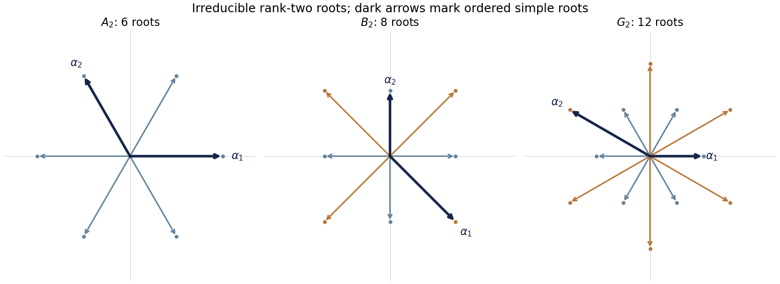
The irreducible rank-two root systems A2, B2 and G2, with long and short roots and explicit ordered simple roots highlighted
. Details. 
Past exam of the mathematics course of the University of Cambridge 2002 iii Paper 63 2 Solution Created 2026-10-03 Updated 2026-10-14
The Kronecker delta is the identity map on the defining representation. Its transformation is . For the alternating Levi-Civita symbol, the determinant identity givesThe lower-index alternating tensor transforms with three inverse matrices and acquires instead. Thus , and are invariant tensors of SU(3). These identities use unimodularity; unitarity identifies the dual representation with the complex-conjugate defining representation.
For a mixed SU(3) tensor representation , the matrix trace is invariant. HencegivesThe trace is the singlet. The traceless matrix transforms by conjugation, so it is the adjoint representation of SU(3). It is irreducible: an invariant complex subspace is invariant under commutators with the complexified algebra , and would be an ideal in that simple Lie algebra. Only the zero and full traceless-matrix spaces are possible.
For the cubic tensor, define its symmetric and antisymmetric first-pair parts byand let be its completely symmetric part. This has independent components and transforms as the symmetric cubic representation of SU(3). Its irreducibility can be seen in the homogeneous cubic-polynomial realization: the simultaneous highest-weight conditions and leave only . A finite-dimensional unitary representation is completely reducible, and each irreducible summand has a highest-weight vector, so this single highest-weight line implies a single irreducible summand. Lowering generates all ten monomials.
Remove this fully symmetric part from , putting . DefineIts trace vanishes because is symmetric in its first two indices. Invariance of makes transform as one upper and one lower index. The inverse map isIndeed contraction with gives . The inverse has the required first-pair symmetry and zero completely symmetric part. Thus this eight-dimensional remainder is another adjoint representation of SU(3).
For the antisymmetric part, defineNow decompose , with traceless. The first term supplies a second independent octet; the trace supplies a singlet proportional to . With , the explicit cubic SU3 tensor projections reconstruct the entire tensor:All projections commute with the SU(3) action because they use permutations and invariant tensors. Their inverse maps and the dimension count establishThe two octets are equivalent as group representations but distinct subspaces in this decomposition; one comes from the first-pair symmetric sector and the other from the first-pair antisymmetric sector. General permutations can mix these equivalent copies.
In the quark model, the up quark, down quark and strange quark form the defining triplet of approximate flavor symmetry. Three-quark baryons therefore have precisely these possible flavor representations. The fully symmetric decuplet corresponds to the observed spin- baryon decuplet: the four Delta baryons, three states, two states and the Omega baryon. Their strangeness rows have flavor hypercharge and isospin ; and occupy the extreme and weights.
The observed spin- baryon octet contains the nucleons, three Sigma baryons, the Lambda baryon and two Xi baryons. In its row, and share the same third-component/hypercharge weight but have different total isospin. Approximate flavor symmetry explains multiplet organization, not exact equality of all their masses: the strange-quark mass and electromagnetic interactions break it.
The two octet copies in the flavor tensor do not require two identical ground-state octets. A three-quark colour singlet is antisymmetric in color; for a symmetric ground-state orbital wavefunction, the Pauli exclusion principle requires a symmetric combined spin-flavor state. The mixed flavor octet tensors combine with the mixed spin- tensors to supply that symmetry. The symmetric flavor decuplet combines with symmetric spin . Together they form the symmetric spin-flavour SU6 representation, with spin-flavor states. A completely antisymmetric flavor singlet cannot appear in this spatial ground state because three spin- indices have no fully antisymmetric spin state: . Three-quark flavour singlet configurations instead require a suitable excited spatial/spin symmetry. Flavor SU(3) here is distinct from the exact color gauge symmetry; treating them as the same group action would misidentify the physical multiplets.
Past exam of the mathematics course of the University of Cambridge 2002 iii Paper 63 1 Solution Created 2026-10-03 Updated 2026-10-14
Use as shorthand for the tensor product of two total-isospin-one states with third components . A total-isospin-zero state must have total third component zero, so write . Applying the total raising operator givesAn isospin singlet must be annihilated by this operator; hence and . Normalization gives the two-isovector singletIt is also annihilated by the total lowering operator. A raising or lowering action changes the third-component label by one; the unchanged output label in the PDF's preliminary ladder formula is a typographical omission, not the action used here.
Exchange commutes with the total isospin operators. The displayed singlet is symmetric. The multiplet has symmetric highest state ; applying the symmetric total lowering operator preserves that exchange symmetry. The symmetric square of a three-dimensional space has dimension six, exactly , while its antisymmetric square has dimension three. The remaining multiplet is therefore antisymmetric. Thus the Clebsch-Gordan decomposition isPions have zero intrinsic spin and form an isospin triplet. Bose-Einstein statistics requires the complete two-pion state to be symmetric under exchange. Its relative orbital state changes by , so odd orbital angular momentum requires antisymmetric isospin: an odd- two-pion state has . This statement treats the charge components as states of the same isospin multiplet, rather than ignoring exchange when their charges differ.
For the decay, let . The stated commutator with gives . More decisively, the commuting raising operator givesThe kaon doublet cannot be raised twice. An component would survive two raisings, so it is excluded. Meanwhile a spinless kaon decaying into two spinless pions has by conservation of total angular momentum, independently of whether parity is conserved by the decay. The exchange condition excludes . This proves the highest-weight weak-isospin selection in kaon decay: the two-pion final state has .
In a consistent pion phase convention, the singlet's charge components have the structureThe normalized symmetric charged channel has coefficient and the neutral channel coefficient . Thus, in the isospin limit with equal pion masses and matching two-body phase space,Equivalently, ordered charged and neutral amplitudes have equal magnitudes, but neutral identical particles contribute the phase-space factor . This is the same counting expressed in another basis, and must not be included a second time after using the normalized charge-channel coefficients. Small pion-mass and electromagnetic effects can modify the ideal ratio.
Past exam of the mathematics course of the University of Cambridge 2002 iii Paper 62 4 Solution Created 2026-10-03 Updated 2026-10-20
The original PDF contains three algebraic misprints in this question. The second internal four-momentum must consistently be , since it is defined by . Its Dirac propagator denominator is , including after contracting the first photon; the printed plus sign is incorrect. Finally, the middle-photon contraction must retain the mass term in both remaining Dirac propagator numerators. The following calculation keeps the electron mass and proves the corrected identities.
Write , and introduceHere is the matrix part of the Dirac propagator, with the overall factors of kept in the common amplitude convention. The Clifford algebra proves . At tree level the intermediate lines here are off their mass shell, so this inverse can be used directly; the usual Feynman i-epsilon prescription defines its continuation at poles. With , the consistently routed tensor isThe external Dirac equations are and .
For the photon at the electron end, and hence . Multiplication by removes that internal line, givingFor the middle photon, . Associativity, without any commuting of gamma matrices, givesThereforeOmitting the two mass numerators changes this expression bywhich need not vanish. For a concrete counterexample take , , and outgoing photon momenta , , . All external momenta are on shell and conserve four-momentum. Choose the upper two-spinor for and the lower two-spinor for , with the other blocks fixed by the Dirac equations. For and , the correct middle contraction divided by is , whereas the expression with the mass numerators omitted is . Thus the printed middle identity is not valid for a massive electron.
At the positron end, . The adjoint Dirac equation gives , so the remaining requested contraction isThe opposite signs at the two ends are precisely what makes the Ward identity work.
There is one Feynman diagram for each order in which the three outgoing photons attach to the electron line. Their orders, encountered from the incoming electron to the incoming Positron, are , , , , and .
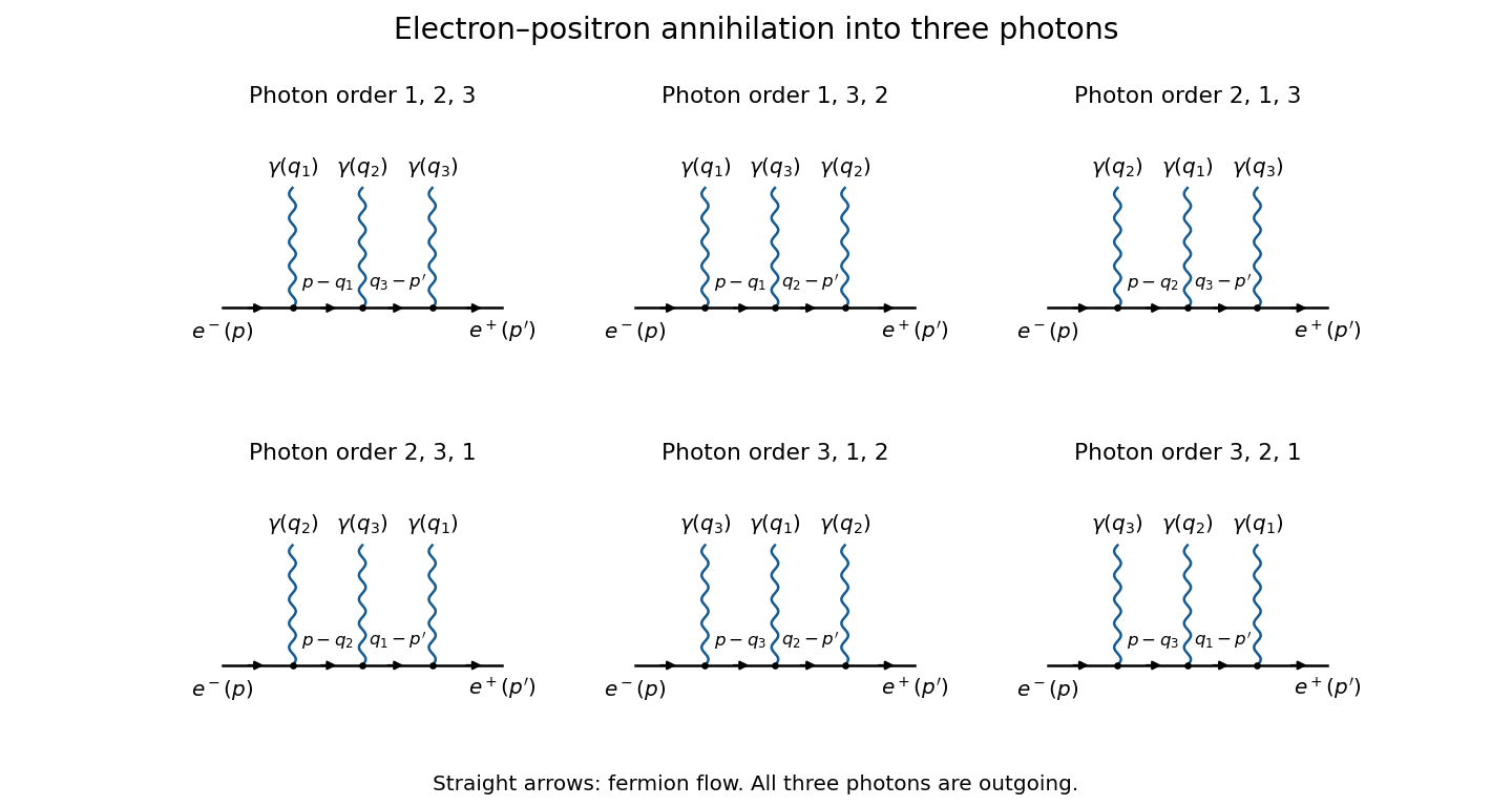
The six tree diagrams for electron-positron annihilation into three photons, ordered along fermion flow
. Details. 
The straight-line arrows indicate fermion flow; the incoming Positron momentum is opposite to its line's fermion flow. Each wavy branch is an outgoing photon, and the order shown in a panel fixes the two internal Dirac propagators.
To prove the full three-photon fermion Ward identity, replace the photon polarization vector of one fixed photon by its four-momentum . Fix the order of the other two photons and write , . There are exactly three positions for photon relative to that order. By the three contractions just derived, their contributions, divided by , areFour-momentum conservation identifies the shared internal momenta in these expressions. The three terms cancel exactly. Repeating for the other order covers all six Feynman diagrams, and provesIndividual Feynman diagrams generally fail this test; their complete sum is essential. By linearity in each photon polarization vector, the result also proves . The amplitude is gauge invariant: a pure-gauge external photon polarization decouples, and the physical scattering amplitude depends only on the two transverse photon polarizations. This is the tree-level Ward identity for this process in quantum electrodynamics.
Past exam of the mathematics course of the University of Cambridge 2002 iii Paper 62 3 Solution Created 2026-10-03 Updated 2026-10-14
Use the Minkowski metric and Feynman slash notation . The Pauli matrices satisfy . In the Dirac representation of the gamma matrices, direct block multiplication givesandThus the spatial anticommutators are , proving the Clifford relationsSince partial derivatives commute, their symmetric product selects the symmetric part of the gamma matrices. Multiplying the Dirac equation by givesHence every spinor component satisfies the Klein-Gordon equation with the same mass.
For parity, let and . The chain rule gives and . Combining these signs with provesThis establishes parity symmetry in quantum field theory for the free Dirac equation, rather than merely asserting its covariance.
A positive-energy plane wave solves . Write . The two block equations areThe second gives . In the first, and make the remaining coefficient zero. There are two independent two-component choices , soFor a massive Dirac spinor, choose as the two rest-frame spin states along a fixed axis, for example . The label distinguishes these canonical spin states after boosting; it is not automatically a helicity label.
Now and for the same fixed . ThereforeThe parity action on canonical massive spin states leaves the canonical spin label unchanged while reversing the momentum. Spin is an axial vector under parity; its orientation is unchanged. Consequently helicity, the projection of spin along momentum, reverses. If had instead been chosen to denote helicity, the transformed label would have the opposite sign.
The Dirac adjoint is , with . ThusThe chirality matrix has in this representation, so and it anticommutes with every . In particular . The parity transformation of a Dirac bilinear therefore yieldsThe first bilinear is a scalar under parity, whereas the second is a pseudoscalar.
For the requested gamma matrix trace identities, use the cyclic property of the trace. Conjugation of a product of gamma matrices by multiplies it by , but leaves its trace unchanged. All odd products therefore have zero trace. Taking the trace of the Clifford algebra relation and using gives . For four factors, move the first gamma matrix successively past the next three using the anticommutators. If , this givesThus . Contracting with the relevant four-vectors proves all four answers:
Past exam of the mathematics course of the University of Cambridge 2002 iii Paper 62 2 Solution Created 2026-10-03 Updated 2026-10-14
For the complex scalar field, the canonical momenta are and . Split . The interaction picture is obtained from the Schrödinger picture by and , choosing a common time origin. The fields therefore obey the free Klein-Gordon equation, while the states evolve through . The canonical quantization of a complex scalar field givesThe adjoint expansion contains and . Particle and antiparticle modes are independent; their nonzero commutators areAll cross-species commutators, and all pairs of creation operators or of annihilation operators, vanish. These formulas reproduce and the remaining vanishing equal-time commutators.
There are no derivative interactions, so the interaction Hamiltonian is . Differentiating the interaction picture state gives . Its time-evolution operator satisfiesIteration gives ordered integration regions . Each is of the full region with a time-ordered product, yielding the Dyson seriesWith the usual asymptotic scattering prescription, taking and provesTime ordering is essential because different interaction Hamiltonians need not commute.
At first order, use the connected tree scattering amplitude, equivalently the normal-ordered quartic vertex with the vacuum and one-particle mass contributions removed. This qualification matters if the local product is interpreted literally without normal ordering: single-vertex tadpole diagrams and vacuum diagrams are not the requested connected two-particle amplitude. The complex scalar quartic contact vertex is obtained fromIn a fully connected matrix element, an incoming particle and outgoing antiparticle attach to the two factors; an outgoing particle and incoming antiparticle attach to the two factors. Each pair has two assignments, giving . The external relativistic normalization of a one-particle state cancels each mode measure: for example and . Consequently the connected integrand is , andThus the invariant connected amplitude isThe Dirac delta function expresses four-momentum conservation.
For the identity contribution, commute through and independently through ; all terms leaving a creation operator against the left Fock vacuum or an annihilation operator against the right Fock vacuum vanish. HenceThere is no exchange term between the two distinct particle and antiparticle species.
Past exam of the mathematics course of the University of Cambridge 2002 iii Paper 62 1 Solution Created 2026-10-03 Updated 2026-10-14
Use units and the Minkowski metric . The canonical momentum of the real scalar field is . Canonical quantization replaces the classical fields by operator-valued distributions and imposes the equal-time canonical commutation relationsThese relations are imposed on an initial slice, with smeared fields understood. In the Heisenberg picture, simultaneous unitary time evolution of both operators preserves their commutators. Since the momentum is , the requested equal-time commutator is .
The Legendre transform in mechanics, applied pointwise, gives the canonical Hamiltonian density of a real scalar field. ThusTo obtain its dynamics rather than assume them, use the Heisenberg equation of motion . The momentum-square term gives . The field-square term gives , while differentiating the Dirac delta function in the gradient term and integrating by parts gives . ConsequentlyBoundary terms vanish for suitably decaying smeared fields. This is the Klein-Gordon equation as an operator identity.
A spatial Fourier transform reduces the Klein-Gordon equation to , where . Its two frequency branches and the Hermitian adjoint condition giveThe invariant-normalized scalar mode extraction can be written particularly simply asSubstituting the mode expansion of a free field proves these inversion formulas: the opposite-frequency coefficient is proportional to and vanishes after spatial Fourier inversion. Alternatively they are the corresponding Klein-Gordon inner products. Taking their commutators using the equal-time fields gives in the mixed case. In the two equal-type cases the delta function enforces , multiplying . ThereforeConversely these mode commutators reproduce : the two frequency contributions each supply half the spatial Dirac delta function.
For the covariant oscillator Hamiltonian of a real scalar field, insert the mode expansion of a free field into . Spatial integration sets the two momenta equal in the mixed terms and opposite in the two-creator or two-annihilator terms. The latter have coefficient . The mixed terms giveThe constant is the divergent zero-point energy; a finite box and a momentum cutoff make its meaning explicit. Normal ordering sets the free vacuum energy to zero and leaves all commutators unchanged. Directly applying the mode commutators to the mixed expression yieldsChoose the Fock vacuum by . Each creation operator adds a boson of energy and four-momentum , while each annihilation operator removes one. Products of commuting creation operators give bosonic statistics from commuting creation operators and unrestricted occupation numbers. The real scalar field has one spin-zero species, identical to its antiparticle. Its one-particle states obey , precisely the relativistic normalization of a one-particle state.
For the Feynman propagator, put and contract the two fields in the Fock vacuum. Only survives, giving the Wightman functionThe stipulated time-ordered product convention is . In a contour integral over , the Feynman i-epsilon prescription places the positive-energy pole just below the real axis and the negative-energy pole just above it. For close below, clockwise, obtaining ; for close above, obtaining . Changing in the second contribution therefore provesActing with multiplies the integrand by . The remaining factor tends to as a distribution, so Fourier inversion givesThe sign also follows from the derivative jump of a free scalar time-ordered two-point function: the first time derivative of jumps by , so that of jumps by .
Past exam of the mathematics course of the University of Cambridge 2002 iii Paper 61 7 b Created 2026-10-03 Updated 2026-10-14
Past exam of the mathematics course of the University of Cambridge 2002 iii Paper 61 7 a Created 2026-10-03 Updated 2026-10-14
Past exam of the mathematics course of the University of Cambridge 2002 iii Paper 61 3 Solution Created 2026-10-03 Updated 2026-10-14
The original PDF prints , with a positive exponent. That premise is insufficient; the intended decay rate is . Indeed every bounded continuous periodic function has . For an explicit counterexample, on setand extend periodically. This is continuous, but for , which is not for any . Thus the sign correction is required in the actual printed question, not just in its converted TeX.
For real continuous -periodic , write for best uniform approximation by degree-at-most- trigonometric polynomials and . A quantitative inverse theorem for trigonometric approximation iswhere is universal. Here is a direct reason for the sum. Choose best approximants and . WriteThe Bernstein inequality for trigonometric polynomials givesFor , monotonicity of best errors bounds by . The first terms are bounded by a fixed multiple of . Also . Nowproves the theorem, for example with a sufficiently large absolute constant .
Suppose, as intended, for , after enlarging to include any finite exceptional indices, where . Since , the inverse theorem givesFor take . Then , so monotonicity of the modulus of continuity and give . For , the separate bound covers the remaining scales. Therefore the corrected conclusion isNow put . The given best approximant to the Weierstrass function leaves the uniformly convergent tail . Its supremum norm is exactly , attained at ; henceThe corrected inverse theorem gives . To show that this order is sharp, set . Every term of is nonnegative, and for the cosine equals because is odd. ThusGiven small , select with . Then . Combining the estimates gives the precise small-scale orderThe exact approximation error can also be verified independently of the supplied fact: at the tail has alternating values . There are enough such points in one period for the trigonometric Chebyshev alternation theorem, since . This is the positive lacunary trigonometric series mechanism behind the best partial sums.
Past exam of the mathematics course of the University of Cambridge 2002 iii Paper 61 2 Solution Created 2026-10-03 Updated 2026-10-14
The relevant uniqueness is uniqueness of the node set, with . Reordering the same nodes cannot change a constraint imposed at every node, so an unsorted “different sequence” obtained only by permutation would not give the claimed counterexample. Order the genuinely different nodes as and let be their Lagrange cardinal polynomials:The denominator has sign . For , repeated differentiation of its numerator givesAll products are nonnegative. At most one factor is zero, and because , some product omits that factor. The derivative is consequently strictly positive, including when , for which the product is empty and equals one. This proves the endpoint derivative signs of Lagrange cardinal polynomials:Choose a single Lagrange interpolation polynomial by prescribing :It satisfies at every prescribed node. Its leading coefficient is , so it has degree exactly . The endpoint sign formula gives simultaneously for all .
Interpolate the Chebyshev polynomial on the same nodes. Since ,The only points at which are its extrema. A different set of distinct nodes includes at least one nonextremal point; at that point the bracket is strictly positive, and so is its derivative weight for every . Moreover : differentiating its differential equation gives , beginning with and ending at . ThusThe same violates every sharp derivative bound, proving uniqueness of Chebyshev derivative-norming nodes for the given Markov-Duffin-Schaeffer theorem. The result concerns node sets or consistently ordered sequences; a mere permutation is the literal ordering exception noted above.
There are unlisted articles, also show them or only show them.