
Past exam of the mathematics course of the University of Cambridge 2002 iii Paper 5 6 Solution Created 2026-10-03 Updated 2026-10-14
Treat as a vector-valued solution; matrix solutions are handled columnwise. It is important to distinguish the coefficient convention from the indicial exponent. In a fixed Fuchsian frame, a finite singularity at meanswhere is holomorphic near . The residue is , equivalently the residue of the matrix-valued one-form . Such a Fuchsian linear differential system has a regular singular point: on sectors, its solutions have at most power and logarithmic growth. Intrinsically a regular singular system can be made Fuchsian by a meromorphic change of frame; a higher coefficient pole in some other frame does not itself prove irregularity. Residues here refer to the displayed fixed coefficient one-form.
At infinity use and . The equation becomesA Fuchsian singularity at infinity means has at most a simple pole at , and . The residue theorem applied entrywise on the Riemann sphere givesFor a direct calculation when all coefficient poles are simple, write by rational partial fractions. Regularity at infinity in this frame requires , so . Transforming coordinates gives . More generally the entrywise residue theorem remains valid even when a different meromorphic frame has higher-order poles.
The printed nonconstant-solution claim is false. A counterexample satisfying its spectral hypothesis isIts residue has eigenvalues , with zero of largest real part. The equations are and . If is analytic at zero, coefficient comparison gives for every nonnegative integer , so . Hence every analytic solution is , which is constant. This disproves nonconstancy, rather than silently replacing it with a weaker conclusion.
A useful correct conclusion is that a nonzero analytic solution exists under the stated hypotheses. Write , and let be the largest nonnegative integer with ; such an exists because . Choose a nonzero and seekThe Frobenius method givesAll left-hand matrices are invertible by maximality of . For large their inverse norm is by a geometric-series inverse; enlarging the constant bounds every by . If on a smaller disc, the scalar majorant with generating functionsatisfies and dominates the recurrence coefficientwise. It converges for , proving convergence of . Thus the analytic solution at a maximal integer Fuchsian exponent is nonzero, and is nonconstant if . When , nonconstancy requires additional information, as the counterexample shows.
There is also a sign problem in the printed exponent terminology. Substitution of with into the actual equation givesThus the indicial exponents are eigenvalues of , not . With the printed sign, an exponent of maximal real part admits a pure Frobenius solution, because the corresponding coefficient matrices are invertible at all subsequent positive integer steps. Lesser exponents can meet resonance.
The supplied example does not demonstrate such failure. Solving it directly givesEvery solution is analytic. The residue eigenvalue corresponds to the true exponent , and setting gives with nonzero leading coefficient. Even with the literal printed factor , every displayed solution has the form with analytic, though .
Nevertheless the last existence-of-a-counterexample request, read literally, can be fulfilled by the diagonal counterexample above. For its nonmaximal residue eigenvalue , substitution of yieldsfor every integer . Neither diagonal entry, or , vanishes, so . Therefore there is no nonzero solution of that literal form, even without imposing .
For the intended logarithmic resonance phenomenon with correctly signed exponents, take insteadIts equation gives and on a chosen branch. The exponent would require , but prevents from being analytic when . The exponent zero has the constant solution . This supplies an explicit resonance obstruction under the correct convention and completes the qualified resolution of the printed defects.
Past exam of the mathematics course of the University of Cambridge 2002 iii Paper 5 5 Solution Created 2026-10-03 Updated 2026-10-14
Take the Jacobi theta functions at zero, with :Define the modular lambda function byThis is an explicit holomorphic expression on the complex upper half-plane. The product formsshow that all three are nonzero there. The theta identity gives , so omits and infinity on the half-plane.
The theta-constant inversion and translation laws, obtained from Poisson summation and changing indices in the defining sums, giveThese formulas imply invariance under the projective groupgenerated by and . This is the effective level-two principal congruence subgroup.
Its action is properly discontinuous because it is a discrete subgroup of . It is also free. An elliptic integral matrix has trace or . The odd traces are excluded because is even. Trace zero would give and , impossible when are even. Thus the only elements acting trivially are the already quotiented central matrices .
A fundamental domain is the ideal quadrilateralwith vertices . The vertical sides are paired by translation by two, and the semicircular sides by . Reduction using these pairings gives the domain; equivalently it is a union of six translates of the standard modular fundamental domain, consistent with the six elements of . On adjoining the cusp points, there are three vertex classes, two paired edges and one face. The resulting orientable compact surface has Euler characteristic , hence is a sphere. This is the compactification of the level-two modular curve.
All three cusp widths are two, so their local parameters are obtained from after a modular change of coordinate. The defining products giveat infinity: there is a simple zero. At the cusp zero, inversion gives , so the value is . At the cusp one, combine inversion and translation; the value is infinity and the pole is simple. The three cusp classes are precisely the parity classes of primitive rational pairs : odd-even, even-odd and odd-odd. A Bézout identity, with parity adjusted by adding multiples of , places any such cusp in the orbit of , or , respectively.
The descended meromorphic function on the compactified quotient thus has exactly one simple pole. Its degree is one, since the degree equals its total pole multiplicity; it is therefore a biholomorphic coordinate on that sphere. Removing the three cusps identifies the quotient with . Consequentlyis a covering map with deck group . The source half-plane is simply connected, so it is the required universal covering map. This proves the universal covering by the modular lambda function, including the absence of interior branching. Three arbitrary distinct punctures are handled by a target Möbius transformation.
Past exam of the mathematics course of the University of Cambridge 2002 iii Paper 5 4 Solution Created 2026-10-03 Updated 2026-10-14
Let be a universal covering map. On a small evenly covered neighborhood in , choose a local inverse of and setAny two such lifts differ by a deck transformation of the disc. Every automorphism of the unit disk preserves the disc density: apply the derivative Schwarz-Pick lemma to the automorphism and its inverse to get equality. Hence the definition is independent of the local inverse. Uniqueness of the universal cover up to a covering isomorphism gives independence of the chosen cover as well. This is the Poincare metric on a Riemann surface, normalized to curvature .
For a piecewise continuously differentiable path , define its length by , and the distance by the infimum of lengths of joining paths. Path reversal and concatenation prove symmetry and the triangle inequality. The distance between distinct points is positive: choose a small closed Euclidean disc around one point not containing the other, on which the positive continuous density is bounded below by . Every joining path must leave that disc and has length at least times its radius before doing so. Joining paths of finite length exist because a plane domain is path connected and the density is locally bounded. Thus this construction gives an actual metric, not just a nonnegative path-length expression.
For the punctured unit disc, use from the complex upper half-plane. The half-plane line element is , while and . ConsequentlyThe domain called an annulus in the paper has inner radius zero, so it is this punctured-disc metric, not the metric of an annulus with positive inner radius.
We now prove the Great Picard theorem. In its holomorphic form, an essential singularity takes every complex value, with at most one exception, infinitely often in every punctured neighborhood. It suffices to prove that a holomorphic function on a punctured disc omitting and extends meromorphically through the puncture: if two values occurred only finitely often, a smaller punctured disc would omit both, and an affine change of target would reduce them to .
Use the universal covering by the modular lambda function , whose construction is given in the following solution. Its deck transformation group is the projective level-two principal congruence subgroup . Rescale the source punctured disc to unit radius. Lift to a holomorphic function . Uniqueness of lifts givesfor a fixed deck transformation . The Schwarz-Pick lemma givesas . A nonidentity deck transformation has no interior fixed point, so it is either a hyperbolic Möbius transformation or a parabolic Möbius transformation. The hyperbolic case is conjugate to a dilation with , . Since , its displacement is at least , contradicting this inequality.
If is the identity, compose with the Cayley transform between the half-plane and disk. Its periodicity lets the resulting bounded function descend to the punctured disc and extend by the Riemann removable singularity theorem. A nonconstant extension takes its central value inside the disc by the maximum modulus principle. The covering map then gives an extension of ; a constant lift gives a constant .
In the parabolic case, its fixed point is a rational modular cusp. Indeed, a parabolic integral matrix of trace has a rational eigenvector for its repeated eigenvalue. Conjugate by an element of the modular group sending this cusp to infinity. The level-two subgroup is normal, so the conjugated transformation is for a nonzero integer . The conjugated lift consequently satisfiesThe modular transformations permute the three target cusp values , as seen from the lambda transformation formulas below. It is therefore enough to examine .
To fix the sign of , the function is periodic in the real direction. Its mean satisfies by the Cauchy-Riemann equations and the increment of . Positivity for all forces . The functionis well-defined, nonvanishing and bounded by one on the punctured disc, so it extends holomorphically to zero. Its winding number along a circle around the puncture is , because a unit increment in increases by . The argument principle therefore shows that has a zero of order at the origin.
At the infinite cusp, the modular lambda function has the convergent expansion in . Thus extends and tends to zero. Undoing the target permutation gives a removable singularity or a pole for . In every case the puncture is not essential, which proves the holomorphic Great Picard theorem. For a meromorphic function with an essential singularity, if three spherical values occurred only finitely often, a Möbius transformation would make the omitted values . The same proof applies because omission of infinity makes the transformed function holomorphic. Hence the meromorphic version has at most two exceptional spherical values.
Past exam of the mathematics course of the University of Cambridge 2002 iii Paper 5 3 Solution Created 2026-10-03 Updated 2026-10-14
For a polygonal domain with finite real prevertices and interior angles , the Schwarz-Christoffel formula has the formwith branches chosen in the complex upper half-plane. A prevertex at infinity is interpreted by the corresponding limiting version of the formula. The exponent records the angle because locally behaves as .
For a slit from to in the upper half-plane, put . The two approaches to its base are separate boundary vertices with angles and , and the tip has angle . With ordered prevertices mapping respectively to the base, tip and base, the Schwarz-Christoffel mapping therefore hasThe tip's factor is a simple zero of the boundary derivative, not an interior critical point.
For the specified power product, the principal branches givethroughout the complex upper half-plane, so maps into that half-plane. Logarithmic differentiation givesThere are no zeros of this derivative in the upper half-plane, so the map is locally conformal there. Its boundary values are negative real for , positive real for , andThe positive scalar factor increases from zero to its maximum at and then decreases to zero, since its logarithmic derivative is . Therefore the tip isThe real boundary runs from the negative real axis to zero, out to , back to zero, and then along the positive real axis.
For completeness, these boundary facts give global injectivity and surjectivity. At infinity,Apply the argument principle on a large upper half-disc, indenting the real prevertices by small semicircles. For a fixed in the upper half-plane off , the limiting image contour is the real boundary with the slit traversed once in each direction, followed by a large upper semicircle. Its winding number about is one. The two slit traversals cancel, so has exactly one zero in the upper half-plane. There are no poles.
Nor can an interior point map onto the open slit. Each point of that slit has two real preimages, one on either side of , with nonzero boundary derivatives. Local continuation across the real line maps the upper half-neighborhoods at these preimages onto the two different sides of the slit. An additional interior preimage would persist for nearby off-slit points and contradict the already proved one-preimage count. The tip cannot be an interior image either: the open mapping theorem would then place nearby open-slit points in the interior image. Finally, never vanishes inside the half-plane. Thus is a conformal bijection onto .
This is the power-product map to a slit half-plane. Its derivative is exactly the Schwarz-Christoffel formula with , , , and . The additive constant is fixed by the boundary value . Thus the power-product expression is an explicit antiderivative of the corresponding Schwarz-Christoffel mapping, with this normalization.
Past exam of the mathematics course of the University of Cambridge 2002 iii Paper 5 2 Solution Created 2026-10-03 Updated 2026-10-14
A normal family of holomorphic functions on a domain is one from which every sequence has a subsequence converging locally uniformly to a holomorphic function, or locally uniformly to infinity in the extended convention. For a bounded family, only finite limits occur.
For functions mapping a plane domain into the unit disc, the Cauchy integral formula supplies uniform derivative bounds on each compact subset. More explicitly, if a closed disc of radius around lies in , the Cauchy estimate gives . A slightly larger compact neighborhood of any given compact set therefore gives uniform boundedness and equicontinuity there. Apply the Arzelà-Ascoli theorem on a compact exhaustion and take a diagonal subsequence. Its limit is locally uniform; the Cauchy integral formula shows that the limit is holomorphic. This proves normality rather than merely invoking it.
Now let on the complex upper half-plane. Every dilation has the same bound, so the argument just given, after scaling the bound if necessary, proves that is a normal family. For any sequence , every locally uniform subsequential limit satisfiesThe identity theorem for holomorphic functions forces . It follows that locally uniformly as : otherwise a sequence violating convergence on one compact set would have a convergent subsequence with this same constant limit, a contradiction.
For , the arc is a compact subset of the complex upper half-plane. Write with . Local uniform convergence of the dilations givesFor the specified sector is empty. This is the same compactness mechanism as the normal-family proof of angular boundary convergence.
To transfer the result to the unit disc, use the Cayley transform between the half-plane and diskIt sends to with , so as . Choose the curvature-minus-one normalization of the hyperbolic metric, for which the disc line element is and the half-plane line element is . The Cayley transform between the half-plane and disk preserves these metrics. For and ,Thus implies . This is the hyperbolic tube around a radial segment estimate. It places in a fixed sector bounded away from the real axis. Moreover implies . Applying the sector result givesA different constant normalization of the hyperbolic metric only rescales and gives the same conclusion.
Past exam of the mathematics course of the University of Cambridge 2002 iii Paper 5 1 Solution Created 2026-10-03 Updated 2026-10-14
For a holomorphic function , the Schwarz-Pick lemma statesEquality in the first inequality for distinct points, or in the derivative inequality at one point, occurs exactly when is an automorphism of the unit disk.
Here is a proof, including the underlying Schwarz lemma. If is holomorphic and , then has a removable singularity at zero. On its modulus is at most . The maximum modulus principle on this circle, followed by , gives and . Equality at a nonzero point, or , forces to be a constant of modulus one by the same maximum modulus principle.
Set , an automorphism of the unit disk. The composite fixes zero. The Schwarz lemma gives the first inequality, while its derivative at zero gives the second. The equality conclusion follows because a composite attaining equality is a rotation. Conversely, every automorphism of the unit disk attains equality. This also proves contraction of the hyperbolic metric.
The boundary lower bound first guarantees a zero inside the unit circle. If , there is nothing to prove about existence. Otherwise, if had no zeros on the closed unit disc, would be holomorphic on a neighborhood of it and satisfy on the boundary. The maximum modulus principle would give , contradicting the hypothesis. The boundary lower bound excludes boundary zeros, so there is a zero with .
The upper boundary bound and the maximum modulus principle give on the unit circle and its interior. The function is nonconstant under the stated hypotheses, so takes its interior values in the open unit disc. Apply the Schwarz-Pick lemma to the points and :This is the zero location bound from Schwarz-Pick, and it applies to every zero inside the unit circle.
The bound is sharp. Given and , chooseThis holomorphic function has no pole in , has constant modulus on the unit circle, and satisfies . With , its zero at gives equality. The case is also attained by .
Past exam of the mathematics course of the University of Cambridge 2002 iii Paper 49 4 Solution Created 2026-10-03 Updated 2026-10-14
Potential-vorticity inversion is the diagnostic recovery of the flow from its advected vortical scalar, using the balance relation and specified boundary conditions. Its usefulness is a separation of tasks: transport the scalar by the current velocity, invert to find the new velocity, and repeat. The inverse is spatially nonlocal even though the transport law is local. The four models differ chiefly in the operator being inverted and the information needed at boundaries.
In two-dimensional vortex dynamics, planar incompressibility permits , and vertical vorticity is . The curl of inviscid momentum givesThere is no vortex stretching in strictly planar motion, so vorticity is materially conserved. The two-dimensional potential-vorticity inversion is the Poisson equation . On the plane, with suitable integrability and far-field behavior, its Green's function is , givingDifferentiation gives the planar Biot-Savart kernel. Here is a harmonic function fixed by boundary, circulation and far-field data. A rigid impermeable wall is a streamline, so is constant on it; constants or circulations around distinct holes require specification. The vorticity alone cannot distinguish two flows differing by a permitted harmonic contribution, such as a uniform current on an unbounded plane. A constant added to has no physical effect.
In nonrotating layerwise-two-dimensional vortex dynamics, strong stable density stratification constrains motion to almost horizontal layers. In the ideal independent-layer limit, vertical velocity vanishes at leading order, andhold separately at each fixed . Height is a parameter: the horizontal inverse Laplacian contains no vertical derivative. With background buoyancy , the leading Ertel potential vorticity is , so the materially advected normalized scalar is . The same horizontal Poisson equation is inverted layer by layer, using each layer's boundary data. This is an asymptotic constrained model, not arbitrary three-dimensional Euler motion with vertical velocity set to zero: its validity requires small Froude number and controlled vertical scales. At finite buoyancy frequency, the weak vertical motion and tilted isopycnals restore coupling. The inversion may be independent by layer while the reconstructed fields vary with height. The horizontal Euler equations for an inviscid fluid determine the pressure gradient, while hydrostatic balance relates its vertical derivative to buoyancy.
In shallow-water quasi-geostrophic inversion, begin with the exact shallow-water potential vorticity . Linearizing its anomaly about depth gives, after multiplying by , . For small Rossby number, geostrophic balance gives , while . Keeping the beta plane background gradient givesThus is inverted with the modified Helmholtz equation , under the specified boundary and far-field conditions. The velocity follows from and surface elevation from . A horizontal Fourier mode of the anomaly satisfiesThe Rossby deformation radius therefore limits the reach of the balanced response. Layer stretching, represented by , is absent from ordinary planar vorticity inversion. Unlike the pure Poisson equation, the finite-deformation operator also responds to the constant part of , which specifies mean elevation rather than an arbitrary streamfunction offset. Specified bottom topography adds a known source to ; it is subtracted along with the background before inversion.
In stratified quasi-geostrophic inversion, continuously varying vertical displacement replaces the shallow layer's single stretching term. For positive and constant nonzero , the three-dimensional quasi-geostrophic potential vorticity isGeostrophic balance and hydrostatic balance give velocity and buoyancy perturbation . Invert the anisotropic elliptic boundary value problem using interior , prescribed top and bottom buoyancy as Neumann boundary conditions, and the lateral, far-field and global-flow data. Boundary buoyancy evolves by its own material conservation when the boundary is impermeable. It cannot be discarded: the Eady edge wave in the preceding solution has zero interior potential vorticity anomaly but nonzero boundary buoyancy and a nonzero induced flow.
For constant , the stretched coordinates for quasi-geostrophic inversion turn the inversion operator into the three-dimensional Laplacian. Its infinite-space Green's function is in coordinates. Hence a horizontal disturbance of scale communicates vertically over scale , explicitly coupling layers. In a bounded domain with homogeneous difference data, multiplying the difference of two inversions by its streamfunction and applying integration by parts givesThis proves uniqueness up to a constant when the relevant boundary terms vanish; a mean or pressure reference fixes the remaining constant. Compatible boundary fluxes are needed for a purely Neumann boundary-value problem.
Across all four models, inversion provides the induced flow, while scalar transport supplies time evolution. The independent horizontal inverse in the first two models becomes a finite-deformation inverse in shallow water and a vertically coupled elliptic inverse in continuous stratification. The principle applies within the stated balance or constrained model. In the unrestricted Boussinesq equations or shallow water equations, gravity waves and divergent motion can share the same potential vorticity, so the vortical scalar alone does not reconstruct every possible flow.
Past exam of the mathematics course of the University of Cambridge 2002 iii Paper 49 3 Solution Created 2026-10-03 Updated 2026-10-14
The basic quasi-geostrophic streamfunction gives , and constant quasi-geostrophic potential vorticity . DefineBecause the background has no potential-vorticity gradient, the linear potential-vorticity equation is simplyIts characteristics have constant , so the general solution is . In particular, is the requested arbitrary separated family; one product is not the most general initial field.
Linearizing the vertical velocity requires retaining advection of by . ThereforeThe impermeable boundary at imposesThis is conservation of boundary buoyancy, not merely a condition that vanish.
For zero interior potential vorticity, write . With , stratified quasi-geostrophic inversion givesThe decaying solution isNo time dependence has been assumed to obtain this vertical structure. Applying the boundary condition gives , henceThus the Eady edge wave travels eastward with horizontal phase velocity for .
The propagation mechanism can be made explicit using boundary parcels. Thermal wind gives the background buoyancy gradient . A small meridional parcel displacement produces boundary buoyancy perturbation . Meanwhile the decaying potential-vorticity inversion gives at the boundary. Consequently there, and the parcel equation becomesA displaced buoyancy contour therefore induces a velocity field that advances that displacement eastward. No interior potential-vorticity gradient is needed because the boundary buoyancy supplies the invertibility data.
Vortex stretching is what sets the induced flow's vertical reach. In the interior, the zero-potential vorticity condition requiresBoundary isopycnal displacement decreases with height as , so fluid columns are stretched or compressed over depth . Conservation of potential vorticity makes this stretching balance the relative vorticity. The resulting inversion factor gives the propagation speed: stronger density stratification reduces penetration and speed, while larger increases them. Zero interior potential vorticity therefore does not imply zero interior flow.
For imposed boundary vertical velocity, retain the same decaying structure and writeThe boundary relation becomes the forced Eady edge wave equationThe integrating factor gives, for ,The arbitrary homogeneous coefficient sets the initial disturbance. With , this is .
At resonance, , integration instead yieldsAn initially undisturbed fluid has . The imposed pumping reinforces the same boundary normal mode every cycle, with no dissipative loss, so the linear amplitude grows secularly. The divergence describes resonance of the undamped linear model; sufficiently large wave amplitude invalidates the assumed small-disturbance approximation.
Past exam of the mathematics course of the University of Cambridge 2002 iii Paper 49 2 Solution Created 2026-10-03 Updated 2026-10-14
Let be layer thickness and gravitational acceleration. The unforced shallow water equations on the equatorial beta plane areLinearize about , . Put and , and scale , , and . Dropping capitals, the linearized shallow water equations becomeThe choice makes both the wave speed and the coefficient of the dimensionless Coriolis parameter equal to one.
Take Fourier modes that decay as . Their equations areFor and nonzero , the first two require . The root gives , and meridional balance becomes . Hence the equatorial Kelvin wave isIt travels eastward at speed in dimensional units. The other sign gives and , so is not trapped.
For , and , inversion of the first two equations gives the equatorial wave velocity polarizationSubstitute in the remaining momentum equation. Multiplication by leavessoWriting yields , the Hermite differential equation. The trapped solutions have the Hermite oscillator quantization and .
For completeness, quantization follows without assuming that every acceptable solution is a polynomial. On decaying smooth functions, define , and . Integration by parts gives and . If , it is an eigenfunction of with eigenvalue . Repeated lowering must terminate: otherwise it eventually produces an eigenvalue below one. At termination , so the terminal eigenfunction is and has eigenvalue one. Repeated raising gives and ; uniqueness of a decaying solution at one end of this second-order equation fixes each mode up to scale.
Thus, away from the exceptional quotients, all fields are determined byInsert this and its derivative in the polarization formulae to obtain and . For , the cubic supplies the low-frequency equatorial Rossby wave and two equatorial inertia--gravity wave branches. Their meridional structures are Gaussian-weighted Hermite polynomials.
For , multiplication by factorizes the equatorial shallow-water dispersion relation asThe physically admissible quadratic gives the mixed Rossby-gravity wave, equivalently the Yanai wave:These fields satisfy all three original equations directly and decay at both infinities, including where the quotient formulae are singular.
To test the other factor, set . The original equations give and . Put ; meridional momentum then givesDecay of at both infinities requires the integral of the right side to vanish. Hence unless . Ordinarily the extra factor supplies no trapped mode. At the exceptional root of the mixed Rossby-gravity mode, , it coincides with the quadratic root and gives the same physical fields, not an additional branch. This distinction avoids discarding a regular physical mode at the crossing.
These arguments concern nonzero wave angular frequency. At , the oscillatory nonzero- modes have , while zero-frequency geostrophic states must be considered in the original equations rather than in expressions divided by .
Past exam of the mathematics course of the University of Cambridge 2002 iii Paper 49 1 Solution Created 2026-10-03 Updated 2026-10-14
Let be kinematic pressure, with the resting hydrostatic part subtracted, and let be the buoyancy perturbation about background buoyancy . The nonrotating inviscid Boussinesq equations, with no buoyancy diffusion, areHere the third equation is mass conservation for incompressible flow, and the last expresses buoyancy conservation following a parcel. Linearization about rest removes the products of disturbances. For a plane internal gravity wave proportional to , the resulting Linearized Boussinesq equations becomeWith and , the first and third equations give . Substitution in vertical momentum and buoyancy gives the dispersion relationSince the velocity is the time derivative of the displacement field, . Thus the complete buoyancy polarization of a plane internal gravity wave isBoth velocity and displacement are perpendicular to the wavevector; pressure and velocity are in quadrature with buoyancy and displacement.
For upward/rightward phase velocity, choose and . Differentiating this dispersion relation gives the group velocity, while the vector phase velocity points along the wavevector:Their dot product is zero and . Draw from the tip of : the right-triangle geometry of internal-wave velocities has horizontal hypotenuse . This hypotenuse is distinct from the horizontal phase velocity .
At an instant with real complex amplitude , write . The spatial fields areThe constant-phase lines of an internal gravity wave slope down to the right, with . Buoyancy maxima lie a quarter wavelength from pressure maxima; the oscillating displacement and velocity run along the phase lines. The group velocity points down and right along them, despite upward/rightward motion of the wave phase.
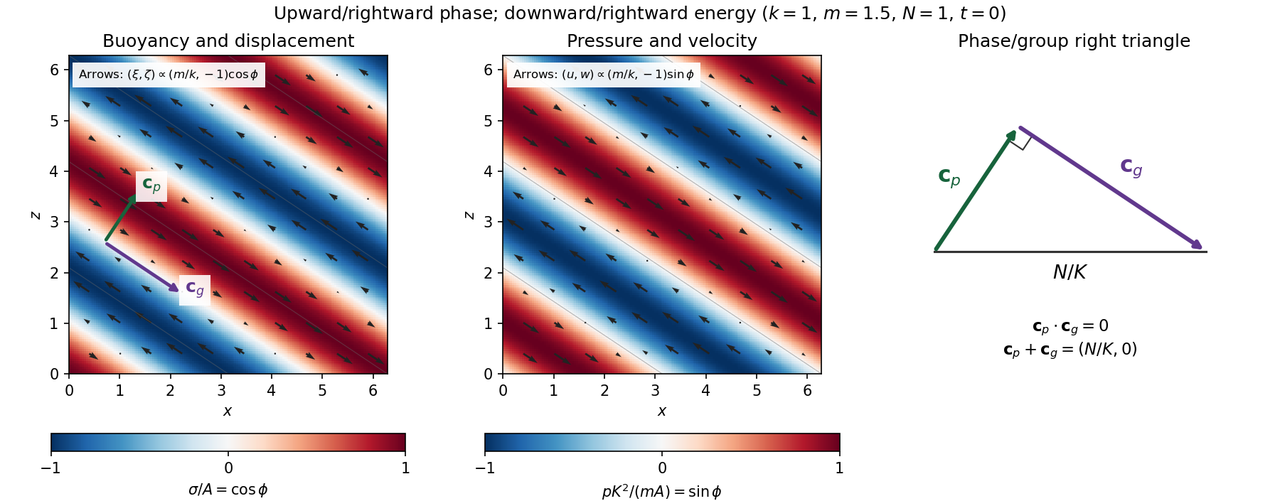
Internal-wave buoyancy, displacement, pressure and velocity fields, with downward energy propagation and the phase/group-velocity right triangle
. Details. 
Let , using horizontal averaging over a wavelength. This is the displacement pseudomomentum of an internal gravity wave, whose sign convention is opposite to . For complex coefficients, . The above wave polarization consequently givesSince , these obey . With weak kinematic viscosity, each leading monochromatic velocity component satisfies , . The dissipative term is therefore , so the supplied averaged balance reduces toFor constant and a steady wave envelope, . As is proportional to squared wave amplitude, viscous attenuation of an internal gravity wave givesHere , so amplitude decreases below a source at : the source is above the receiving level. The same conclusion follows directly because downward group velocity carries energy from the source downward. Upward phase velocity does not locate the source.
For a slowly varying mean shear flow , the local intrinsic frequency is . A local WKB approximation uses , with varying vertical wavenumber and group velocity. The appropriate transported quantity is wave action, or horizontal wave pseudomomentum ; its vertical flux has viscous loss, and the changing polarization factors must be retained. In particular, is no longer constant.
Near a critical level of an internal gravity wave, , so and . The damping per vertical distance, of order , grows rapidly. The waves are strongly attenuated over a narrow altitude range and transfer momentum to the mean flow there or before reaching the critical level. The inviscid WKB approximation eventually fails; viscosity and possibly internal-wave breaking regulate the small scales.
Past exam of the mathematics course of the University of Cambridge 2002 iii Paper 48 4 Solution Created 2026-10-03 Updated 2026-10-14
Write and . The forcing acts on the fast initial-time scale, so first remove a localized particular solution. Expanding the coefficient there givesA particular choice is , henceIts initial value is and its initial derivative is . The localized forcing determines WKB phase constants; omitting it before imposing the initial conditions would miss the permanent free oscillation.
For the homogeneous part, the slow-time equation is . Write its WKB approximation as , normalizing . The leading amplitude transport equation gives and leading phase .
To include every contribution on bounded slow-time intervals, the first phase correction is needed. If the local phase wavenumber is , the real part of the amplitude-phase equation gives . The WKB phase correction for a slowly varying oscillator, anchored to zero at the initial time, is thereforeThere is no first-order bulk amplitude correction in this normalization. At , the homogeneous initial value must be and its initial derivative . Since and , these give and . The requested forced approximation isfor with fixed . The approximate initial value is exactly one through this order and its derivative is . The particular-solution residual is uniformly localized and ; the corrected homogeneous residual is on the long interval, producing solution error after integration over times of order .
The WKB approximation requires the relative frequency-change parameterIt therefore fails when , even though the coefficient has no finite-time zero. This is the Bessel transition for an exponentially decaying oscillator. Introduce the shifted slow time and amplitudeThe exact rescaled equation isFor fixed its right side is smaller than every algebraic power of . The leading transition problem is consequentlyWith this becomes , the order-zero Bessel differential equation. This identifies the governing equation without solving it.
The amplitude-phase series also supplies overlap data while , although its bounded- absolute error estimate is not uniform up to the transition. For matching, combine the earlier sine and cosine terms into through first order. In the overlap , their phase isto the retained order. Thus amplitude and phase matching as requireThese are oscillatory amplitude-phase conditions, rather than pointwise ratio statements at zeros. The smaller phase term records the first overlap correction if required. The rapidly varying matching constant must be retained as data; there is no single epsilon-independent limiting phase. The two matching conditions determine the leading transition solution, which is deliberately left unsolved.
There are unlisted articles, also show them or only show them.