
Past exam of the mathematics course of the University of Cambridge 2002 iii Paper 67 5 Solution Created 2026-10-03 Updated 2026-10-14
The RNS string adds worldsheet Majorana fermions to the coordinate fields . The new fields are spinors on the worldsheet but vectors under the target Lorentz group; this distinction matters when interpreting their oscillator states. In a flat target, a convenient Lorentzian convention for the free gauge-fixed action iswhere are two-dimensional gamma matrices. The bosonic and fermionic kinetic terms are related by worldsheet supersymmetry. Before fixing local worldsheet supersymmetry, one introduces a worldsheet gravitino along with the worldsheet metric. After superconformal gauge fixing, the residual matter constraints are the Virasoro constraints and the constraints generated by the superconformal current .
Each real worldsheet Majorana fermion contributes to the chiral central charge, while each coordinate contributes one. The reparameterization bc system contributes , and fixing local worldsheet supersymmetry also produces commuting superconformal ghosts of weights , with central charge . ThusIn light-cone gauge in string theory there are eight physical transverse coordinate fields and eight transverse worldsheet Majorana fermions.
On the doubled spatial interval of an open string, the two allowed fermionic periodicities areThey arise from the relative signs of the left-right fermion gluing conditions at the two ends. Thus the Ramond sector has integer-mode oscillators , including , and the Neveu–Schwarz sector has half-integer oscillators , , without zero modes. In either sector,A closed string has independent left- and right-moving periodicities, giving four sector choices rather than two.
The Ramond zero-mode Clifford algebra isHence its ground states carry a Spinor representation of the Lorentz group. The zero-mode supercurrent constraint reduces on a ground state to the Dirac equation . In the Neveu–Schwarz sector the oscillator vacuum instead carries a scalar representation. Consequently the open string NS sector describes spacetime bosons, while the R sector describes spacetime fermions. Exciting a target-vector oscillator does not change this statistics assignment.
The string intercepts follow from the transverse zero-point energy. Per boson the integer-mode contribution is . Per fermion it is the negative of the corresponding half-sum. Since , the eight transverse pairs giveThus , , and the open string mass formula is . This distinguishes the lowest states explicitly:
- In the NS sector, the level-zero scalar is a tachyon with . At level , is a massless vector. The supercurrent and Virasoro constraints give and the equivalence . There are eight physical vector polarizations.
- In the R sector, the level-zero states are massless spacetime spinors satisfying the Dirac equation. Before the GSO projection, the two chiralities together give 16 on-shell polarizations; they split into the two eight-dimensional transverse spinor representations.
The supersymmetric GSO projection keeps odd oscillator fermion number in the NS sector. Defining so that the NS vacuum has , its projector isIt removes the scalar tachyon and keeps the massless vector. In the R sector, fermion parity contains the zero-mode chirality operator, so one may writeHere counts nonzero-mode fermionic excitations. On the ground states, this keeps one Majorana-Weyl spinor chirality: 16 real covariant components, or eight on-shell polarizations after the Dirac equation. The projected massless open-string states are an eight-polarization gauge vector and an eight-polarization gaugino. The compatible projected tower exhibits spacetime supersymmetry; unprojected worldsheet supersymmetry by itself did not eliminate the tachyon or equalize these massless counts.
For a closed string, both chiral zero-mode constraints must hold:This shifted closed-string level matching is particularly important in the mixed sectors. The lowest states and their spacetime nature are as follows.
- The NS-NS sector is bosonic. Before projection, is a scalar tachyon with . The GSO projection on each side removes it. The surviving lowest level is , with transverse states . Decomposing their tensor product into symmetric traceless, antisymmetric and trace parts gives the graviton, Kalb–Ramond field and dilaton, with physical polarizations.
- The RR sector is bosonic, since it combines two spacetime spinors. Its lowest states have and are massless. The two Dirac equations on the bispinor polarizations identify them with on-shell differential-form field strengths. After projection they supply 64 bosonic polarizations. The actual form degrees depend on the two chosen Ramond sector chiralities.
- The NS-R sector and R-NS sector are fermionic. Their respective lowest level-matched pairs are and , not two oscillator vacua. A vector tensored with a chiral spinor decomposes into its gamma-traceless vector-spinor and gamma trace. These give a massless gravitino and dilatino, with polarizations in each mixed sector. The vacuum pair would fail the shifted closed-string level matching, so it cannot be counted as a mixed-sector tachyon.
For type IIA superstring theory, the two R sector ground-state chiralities are opposite. The Ramond–Ramond potentials can be represented by , with transverse counts . The two mixed-sector gravitinos have opposite chiralities, and the ten-dimensional theory is nonchiral. For type IIB superstring theory, the two R sector chiralities agree; the Ramond–Ramond potentials are , with self-dual five-form field strength, giving . Its two gravitinos have the same chirality. Thus both projected type II theories have 128 massless bosonic and 128 massless fermionic polarizations and no tachyon, while their chiralities and form spectra differ.
If unoriented open strings are included in the complete theory, the supersymmetric example is type I string theory. Worldsheet orientation reversal projects the closed type IIB superstring theory spectrum and identifies the two mixed sectors; the surviving closed fields include the graviton, dilaton, a Ramond–Ramond potential , and one gravitino and dilatino. The open states form vector and gaugino multiplets with Chan-Paton factors; tadpole and anomaly cancellation select . This is an additional orientation projection, not part of the GSO projection itself. The heterotic string instead pairs one supersymmetric chiral side with a bosonic chiral side carrying an internal gauge sector; it does not have a Ramond choice on both sides.
Past exam of the mathematics course of the University of Cambridge 2002 iii Paper 67 4 Solution Created 2026-10-03 Updated 2026-10-14
Let be the compact coordinate, identified modulo . The closed string may wrap the circle:Single-valued momentum eigenfunctions require , . These are the momentum and winding modes. Write the chiral zero-mode momenta asThe left-moving string oscillators will be tilded: , . This fixes the sign in compact-circle closed-string level matching.
Define the lower-dimensional mass by . The two closed-string physical-state Virasoro conditions, with bosonic string intercept one, areTheir average and difference derive the complete free bosonic string mass spectrum on the circle:The allowed states have nonnegative integer oscillator levels and obey the Virasoro constraints within each chiral sector. Compactification has not removed oscillator polarizations; it has added quantized compact momentum and allowed winding while changing the lower-dimensional interpretation of those polarizations.
At large , the momentum and winding modes with have closely spaced momentum energies , whereas nonzero winding costs . At small their roles reverse. The precise equality is T-duality:It leaves unchanged and reverses , and leaves the mass formula and closed-string level matching unchanged. On the string embedding map it reverses the right-moving part of . Therefore the small-radius spectrum is the large-radius spectrum of the dual theory, rather than a spectrum in which all charged states simply become heavy.
At a generic radius, the neutral level contains the lower-dimensional graviton, Kalb–Ramond field and dilaton, two gauge bosons from the mixed components of the metric and two-form, and the radius modulus of a string compactification. The two vector charges are the Cartan charges of .
Consider instead the following charged states:Every state satisfies compact-circle closed-string level matching. The single noncompact string oscillator supplies a vector polarization. At the massless point, the level-one Virasoro constraint imposes transverse polarization and its physical null string state identifies polarizations differing by the noncompact momentum. Thus these are genuine lower-dimensional vector states. Their squared mass isThus four additional charged massless spin-one particles appear atFor the charges have , ; for they have , . This identifies the two pairs of charged roots.
The enhanced gauge group can be derived rather than just inferred from counting. At the self-dual circle, the chiral compact boson satisfies . The self-dual circle current algebra has currentsThe exponentials have conformal weight . Free-boson contractions give the operator product expansionsThey form the level-one SU(2) Lie algebra, and there is an independent right-moving copy. The string vertex operators and give the six massless vectors. ConsequentlyChanging gives the four charged vectors the mass found above, consistent with the radius deformation as a Higgs mechanism.
For completeness, the enhanced spectrum also has scalar fields. Using a compact rather than noncompact oscillator in the four singly excited charged families gives four scalars. At , closed-string level matching requires ; the mass equation then gives the four charges . These exceptional massless ground states of a bosonic circle give another four scalars. Together with the radius scalar they form nine scalars in the representation, in addition to the neutral dilaton. The ever-present neutral bosonic tachyon still has . The enhancement establishes the additional massless vectors, not stability of the entire bosonic vacuum.
Past exam of the mathematics course of the University of Cambridge 2002 iii Paper 67 3 Solution Created 2026-10-03 Updated 2026-10-14
The Polyakov action introduces an independent worldsheet metric :Its redundancies are worldsheet diffeomorphisms and Weyl transformations. A Polyakov path integral over all metrics without dividing by this gauge volume would count physically equivalent configurations repeatedly. Fixing conformal gauge therefore needs the Faddeev-Popov determinant, not merely the substitution of a flat metric into the action.
After using the Weyl transformation to remove the trace of a metric variation, the infinitesimal worldsheet diffeomorphism ghost operator isThe Faddeev-Popov determinant of this operator is represented by anticommuting fields: a vector Faddeev-Popov ghost and a symmetric traceless Faddeev-Popov antighost field . In Euclidean coordinates their worldsheet ghost action is, up to a consistent overall normalization,The two chiral copies of this bc system have conformal weights and anticommutators . They are auxiliary fields for the gauge determinant, not additional spacetime particles. Their use is different from the unwanted timelike negative-norm string states of covariant matter quantization.
The chiral holomorphic stress-energy tensor of the bc system isDouble contractions in its operator product expansion give the central charge of reparameterization ghosts . Equivalently, a fermionic bc system with antighost weight has , and gives . The free coordinate matter contributes . Thus the total worldsheet Weyl anomaly vanishes for the flat critical bosonic string theory precisely whenThis statement assumes no additional matter or compensating Liouville field theory.
BRST symmetry expresses the gauge symmetry after gauge fixing by replacing its infinitesimal parameter with the Grassmann variable . In one chiral conformal patch, its graded action has the formthere is an analogous barred copy for a closed string. The Grassmann parity makes : the term from cancels the term from applying to , while the term with vanishes. The gauge-fixed chiral transformations are on shell when their conservation equations are used. At the quantum level, BRST nilpotence also tests the anomaly.
For example, an open string BRST charge can be written using the matter Virasoro generators asUse the ghost oscillator vacuum and the corresponding oscillator normal ordering. In this convention the last term is in the critical theory. With a differently shifted ghost , the displayed intercept must be shifted consistently; one must not count the same shift twice. Squaring shows why both critical conditions are needed. Its anomalous terms, in this convention, have coefficientsThe independent cubic and linear terms vanish at , . The equivalent chiral BRST current is , with its contour integral defining the charge.
The graded identity recovers the gauge constraints. In particular, on , BRST-closed imposes and . Physical states are classes in BRST cohomology,at the appropriate ghost number: one for the usual open-string vertex and two for the closed-string vertex, with the closed-string zero-mode and closed-string level matching conditions also imposed. Since , an exact shift preserves closure. BRST Ward identities make exact insertions decouple from physical amplitudes and establish gauge independence. Together with the no-ghost theorem for the critical bosonic string, this explains how the auxiliary ghosts enforce gauge invariance while the physical spectrum retains positive norm.
Past exam of the mathematics course of the University of Cambridge 2002 iii Paper 67 2 Solution Created 2026-10-03 Updated 2026-10-14
The Nambu–Goto action is invariant under worldsheet diffeomorphisms. Its canonical Nambu–Goto phase-space constraints areIn conformal gauge, , so these become . Their smeared generators implement the residual conformal transformations rather than independent propagating degrees of freedom. Classically their Fourier modes form the classical Virasoro constraint algebra. Quantization promotes them to the Virasoro algebra, and its constraints select the physical string states from the indefinite covariant Fock space.
For clarity, start with a Neumann boundary condition at both ends of an open string, . Its open-string mode expansion isCanonical quantization gives the string oscillator relationsWith , the worldsheet stress-energy tensor obeysSubstituting the open-string mode expansion into this quadratic expression derives the Virasoro generators:The colons mean normal ordering, placing the negative-mode creation operators to the left. The string level operator increases by when an oscillator is added.
Using the commutator once givesApplying this to the quadratic expression for produces , together with the double-contraction Virasoro central extension. To determine its coefficient, take and evaluate on a zero-momentum oscillator vacuum. Only the creation pairs with contribute, givingHere is the target spacetime dimension; the timelike free boson also contributes one to the central charge, since a double contraction contains two metric factors. ThusThis derives both the Virasoro generators and their quantum anomaly.
In old covariant string quantization, the physical-state Virasoro conditions for an open string arewhere is the normal-ordering constant of a string. Requiring all positive and negative modes to annihilate a state would contradict the nonzero Virasoro central extension; the positive-mode prescription is the appropriate covariant subsidiary condition. The zero-mode equation gives the open bosonic string mass spectrum,For a closed string, there are two commuting Virasoro algebras. With uncompactified zero modes, and . Imposing both positive-mode conditions and both zero-mode conditions gives the closed-string level matching and .
Covariance initially retains the timelike string oscillators. For example, has negative norm because . Its existence in the unconstrained space is not an inconsistency if it is absent from the physical quotient. The no-ghost theorem for the critical bosonic string states that, at and , the inner product on physical string states at ordinary nonzero momentum is positive semidefinite. After quotienting physical null string states, this physical space is represented by the 24 positive-norm transverse string oscillators.
A spurious string state has the form . Its inner product with every physical string state vanishes, by and . Whenever such a state is itself physical, it is a null string state and represents a gauge redundancy, not an extra polarization. Consequently the physical quotient has no negative-norm propagating states, and agrees with light-cone gauge in string theory. This is the significance of the theorem; a proof is not needed here. It does not eliminate the bosonic tachyon, whose negative mass squared is distinct from negative norm, nor does it remove the auxiliary worldsheet ghost fields used in gauge fixing.
Past exam of the mathematics course of the University of Cambridge 2002 iii Paper 67 1 Solution Created 2026-10-03 Updated 2026-10-14
Use Minkowski spacetime with signature , and write the string tension as . If is the string embedding map, its induced worldsheet metric is . The Nambu–Goto action isThe first variation uses and therefore givesAn integration by parts yields the bulk Nambu–Goto equations of motion and the endpoint term:For a closed string, periodicity cancels the endpoint term. For a freely moving open string, arbitrary endpoint variations require zero momentum flux, which is the free-end string boundary condition.
Choose orthogonal conformal coordinates on the nondegenerate part of the worldsheet, so that and . The Nambu–Goto equations of motion then become a wave equation, with the accompanying Virasoro constraints:Here a dot and a prime mean and . The last two equations are essential: a solution of the wave equation alone need not be a relativistic fundamental string motion.
For a free-ended open string, take and , and setwith the other coordinates constant. Every component satisfies the wave equation, andMoreover at both endpoints, giving the Neumann boundary condition. At fixed target time , the spatial image is the straight segmentThus its angular velocity is . The speed at coordinate is , so the endpoints have the null motion of a free string endpoint. The induced worldsheet metric degenerates there; the conserved densities below have finite limits, so the endpoint degeneracy causes no divergent charge.
In these coordinates . The target-space Noether charges of a string give the energy, momentum and angular momentum:Since this is the centre-of-momentum frame, the rest mass is . Eliminating proves the free-ended straight-string Regge relation:A spacetime Lorentz transformation of the solution changes its frame, not this rest-frame relation.
There is also a folded closed string version: use the same formula over . The spatial segment is then covered twice, with folds at , and the closed-string mode expansion is periodic. Each charge is twice its open string value, soThe folds also have degenerate induced metric and are understood through the finite canonical densities or a limiting smooth motion. The two classical Regge trajectories have different slopes because the closed string has two coincident branches. No quantum string intercept enters this classical calculation.
Past exam of the mathematics course of the University of Cambridge 2002 iii Paper 66 3 Solution Created 2026-10-03 Updated 2026-10-14
Let be Hermitian color generators with , and take . In explicit spinor, color and flavor indices the massless kinetic term isThe full Quantum chromodynamics Lagrangian also has . A local color gauge transformation acts asThus and the kinetic term is gauge-invariant.
Since the gauge coupling is independent of flavor and chirality, the classical internal global transformations are , , with constant flavor matrices . Equivalently these consist of , a common vector phase, and a singlet axial phase , modulo shared discrete factors. The vector phase measures quark number, or baryon number after dividing its generator by three. The nonsinglet axial rotations may be written . At the quantum level the singlet axial phase is anomalous; the exact continuous internal symmetry is up to those discrete identifications. The usual spacetime Poincaré transformations also leave the theory invariant; the massless classical theory has dilation symmetry, which is broken by quantum running. These distinctions are massless two-flavor QCD symmetries.
At equal time the canonical relations, including all indices, areNo constraint removes any of the four spinor components of the Dirac field in these equal-time relations.
To evaluate the axial charges, first prove the elementary bilinear identity. For any constant matrix on the spinor/flavor space,For example ; the spatial delta function collapses the integral. This proves the charge action directly from the canonical anticommutation relations.
For , anticommutation of and then givesThe charge is an even operator, so its commutator obeys the ordinary product rule. ConsequentlySimilarly, using and the Pauli matrices identity ,Composite fields can be defined with a common symmetry-preserving regulator; these nonsinglet identities have no color axial anomaly. This is the nonsinglet axial charge algebra of quark densities.
If every conserved axial charge left the vacuum invariant, the vacuum expectation of each such commutator would vanish. A nonzero quark chiral condensate instead makes for . It therefore diagnoses spontaneous breaking of the nonsinglet chiral symmetry. In the massless two-flavor limit, the observed hadronic pattern is described by , with three Goldstone boson modes identified with the pions. The vacuum condensate is a dynamical property of QCD, not something derivable from the canonical algebra alone. The light pion multiplet and absence of parity-degenerate light hadrons support this pattern; the singlet axial anomaly prevents interpreting an additional singlet mode as a fourth Goldstone boson.
For equal nonzero masses, add . It is invariant under local color gauge transformations and common vector flavor rotations, but not under independent left/right rotations. The exact continuous flavor symmetry becomes . The kinetic term and canonical anticommutators are unchanged, and the two proved equal-time commutators still hold. The charges, however, are no longer conserved:The first equation follows from the massive Dirac equations, or the last from and . This is the flavor-nonsinglet axial Ward identity with equal quark masses. The pions become pseudo-Goldstone bosons with , rather than exact massless modes. To leading order, in the convention , . The condensate persists for small masses, but the symmetry is now explicitly broken, so the exact-symmetry Goldstone argument is replaced by an approximate one. The singlet anomaly and gauge symmetry are unaffected.
Past exam of the mathematics course of the University of Cambridge 2002 iii Paper 66 2 Solution Created 2026-10-03 Updated 2026-10-14
Take metric and write . The outgoing electron and antineutrino momenta are and . Up to an irrelevant overall phase, the amplitude isA fermion spin sum givesAnticommuting through the massless momentum and gamma matrix, and using , reduces the trace to twice the four-gamma trace minus twice its counterpart. In particular its symmetric part isThe epsilon-tensor part is antisymmetric and contributes neither to the unpolarized polarization sum nor to the real linear polarization used below. There is no extra factor for selecting the neutrino helicity: the chiral vertex has already done so.
The external massless equations imply for , so . With , averaging over the three initial spin states givesIndeed . This is a massive-vector spin average, not an average over the final spins.
In the rest frame, eliminating the momentum delta function and integrating the remaining radial delta function reduces the two-body Lorentz-invariant phase space to . ThereforeThis derives the massless leptonic W decay width without invoking a precomputed decay formula.
For the specified polarization there is no initial spin average. Put , and . The contraction selectsIt follows thatHere . The total rate agrees with the spin-averaged result, but its normalized polar distribution is instead of the isotropic unpolarized distribution. This is polarized massless leptonic W decay.
Past exam of the mathematics course of the University of Cambridge 2002 iii Paper 66 1 Solution Created 2026-10-03 Updated 2026-10-14
Use and . For each generation , the leptons areBoth are color singlets. The conjugate antilepton fields transform in the conjugate representations and have opposite hypercharge; they are already included by the conjugate fields in the Lagrangian. The two components of have electric charges , and has charge . There is no right-handed neutrino representation in this field content. These assignments use the electroweak representation and hypercharge table in the same hypercharge normalization as the scalar doublet.
For a doublet of hypercharge , defineThe term is absent for a singlet. Under the local transformation , the gauge fields transform so that . Consequently the required gauge-covariant kinetic terms areThe fields of definite chirality are defined with . Since has hypercharge , the Yukawa interactionis invariant: its hypercharges add to zero, and contracts the two doublet indices. A bare charged-lepton mass violates these assignments. No renormalizable neutrino Yukawa term is available without a right-handed neutrino. A gauge-invariant scalar potential depending on can select the nonzero vacuum, without altering these kinetic and Yukawa constructions.
There is an explicit local unitary gauge transformation whenever :Thus, with the real field ,This proves the polar coordinates for the electroweak Higgs doublet constructively. The gauge choice is local about the nonzero vacuum; it need not be nonsingular at zeros of the doublet.
The three identical-generation kinetic terms permit unitary flavor changes. A singular value decomposition gives with . Rotate both components of each left doublet together, and the right singlets independently. In this basis,The left/right cross terms combine into this Dirac mass. Since the neutrinos have no mass matrix, their simultaneous left rotation preserves a diagonal charged current. This is charged-lepton Yukawa matrix diagonalization; the neutrinos remain massless in the stated renormalizable model.
The scalar kinetic term givesIntroduce and . The combinations , , and therefore diagonalize the quadratic terms:The factor applies to the real neutral field, not to the complex charged field. The massless photon corresponds to the unbroken generator , which annihilates the vacuum. This gives the electroweak doublet gauge-boson mass matrix and its diagonal spectrum.
Past exam of the mathematics course of the University of Cambridge 2002 iii Paper 65 4 Solution Created 2026-10-03 Updated 2026-10-14
Absorb the gauge coupling into the connection and use . The anti-Hermitian generators make unitary for real parameters. With a matter field transforming as , require . Applying both sides to an arbitrary field givesExpanding and yields the infinitesimal gauge transformation with an anti-Hermitian connectionThe adjoint covariant derivative is . In components,The trace normalization makes the structure constants totally antisymmetric: and cyclicity of the trace supply antisymmetry in the remaining indices. Replacing by reverses the infinitesimal parameter convention and gives ; mixing the two conventions would change the ghost operator incorrectly. The trace normalization also gives the invariant quadratic form .
A gauge-invariant functional integral counts all representatives along each gauge orbit. The gauge condition selects a representative, and its delta functional enforces that selection. Assume a local patch where each orbit intersects the gauge slice once and the gauge-condition derivative has no residual zero modes. DefineChanging the orbit integration variable from to givesInsert this Faddeev-Popov gauge-orbit identity into the unfixed path integral. The action and measure are invariant under a change , so integration over factors out as the gauge-group volume. Dividing by that redundant volume leaves the fixed integral and its Faddeev-Popov determinant. In a perturbative patch with fixed determinant sign or phase, the absolute value is replaced by the oriented determinant, up to a field-independent normalization:Here . This is a functional determinant of the gauge-condition Jacobian, not an arbitrary extra weight. The local invertibility assumption matters: residual gauge transformations or multiple orbit intersections, described by the Gribov ambiguity, prevent treating this derivation as a global unique gauge slice without further qualifications.
Both extra factors can be incorporated into an enlarged action. An auxiliary real field Fourier-represents the delta functional, while a Grassmann Gaussian integral over independent Faddeev-Popov ghost fields represents the determinant:Thus the original fixed integral can be written with action and ordinary integration over the extra fields, with no explicit delta functional or determinant. The anticommuting fields give a determinant rather than the inverse determinant obtained from commuting Gaussian fields.
For the usual Gaussian family of gauges, add and integrate out . Completing the square producesThis is Gaussian gauge fixing with an auxiliary field; equivalently one averages the condition with its Gaussian weight. Gauge-invariant observables are unchanged apart from normalization. For the Lorenz gauge , the chosen transformation convention gives . The ghost action is , or after integration by parts. The dependence of on accounts for the ghost interactions.
Past exam of the mathematics course of the University of Cambridge 2002 iii Paper 65 3 Solution Created 2026-10-03 Updated 2026-10-14
The renormalization-group beta function isAt one-loop accuracy, integrating givesFor a positive weak coupling and , the coupling increases toward the ultraviolet and decreases toward the infrared. Extrapolation predicts a Landau pole at , where the weak-coupling approximation fails. For , the positive coupling decreases toward zero as : this is asymptotic freedom. Toward the infrared it instead grows, so perturbation theory eventually fails. The zero coupling is a fixed point. If negative couplings are allowed mathematically, their direction of motion still satisfies , but the side on which the pole occurs reverses: for example approaches zero from below in the ultraviolet. Negative quartic coupling does not give a stable scalar potential.
For the loop calculation use , , and the PDF's vertex normalization . A Feynman parameter combines the denominators. Shift the Euclidean loop momentum to , and put . The regulated integral without the vertex prefactor isUsing Schwinger parameterization, , and the momentum Gaussian integral givesFor , , while the other factors have finite limits. Thus the massive scalar bubble pole in four dimensions isThis pole is independent of external momentum and mass and hence is canceled by a local quartic counterterm. There are three channels, corresponding to the three pairings of four external momenta. Their poles add, and a counterterm vertex cancels the sum whenThis is the total counterterm for the three four-point diagrams specified here. The minimal subtraction scheme removes their poles only. The one-loop tadpole is momentum independent and requires a mass counterterm, but does not produce one-loop wave-function renormalization; that is why it does not alter this one-loop coupling calculation.
The dimensionful bare coupling is thereforeIts independence of givesPutting , the finite coefficient of is . ThusThis is the one-loop quartic scalar beta function, positive for nonzero weak real coupling. The factors would look different with a regulator , but the four-dimensional beta function is unchanged. For massless theory take nonexceptional external momentum, or an infrared regulator, so an infrared singularity is not confused with the ultraviolet pole.
Past exam of the mathematics course of the University of Cambridge 2002 iii Paper 65 1 Solution Created 2026-10-03 Updated 2026-10-14
Use metric signature and initially set . For an internal scalar line with momentum , the Feynman propagator is . An -leg Feynman vertex, for , contributes , with all incident momenta incoming. Its in the Lagrangian density is canceled by the permutations of its identical fields. Each vertex conserves momentum and supplies . Integrate each independent loop momentum with , multiply the line and vertex factors, and divide by the Feynman-diagram symmetry factor for labeled external legs. Sum the distinct graphs and external-momentum assignments without counting the same assignment twice.
An unamputated momentum-space correlation function also contains the external propagators. Dividing the generating functional by its zero-source value removes disconnected vacuum bubbles; taking its logarithm selects connected correlation functions. Amputation of external propagators removes the external line factors when computing vertex amplitudes. Translational invariance leaves one overall momentum-conservation delta function for each connected graph.
The loop order is the number of independent graph cycles, equivalently the number of independent momentum integrations left after vertex conservation. A spanning tree through interaction vertices contains internal edges; hence, with internal lines,Restoring in gives for each internal propagator and for each interaction vertex. Thus an amputated connected amplitude hasThe same counting holds for a diagram in when the external source is coupled as : every external propagator brings , canceled by the source insertion's . This is Planck-constant loop counting with source normalization. An ordinary connected expectation of fields, with no such source factors, instead scales as ; multiplying by to form shifts its source-kernel counting to . The normalization must be specified when applying the printed loop rule.
Let count -valent interaction vertices. Counting their incident half-edges gives . Substituting the loop identity yieldsEach coefficient on the right lies between and , proving the vertex-count bounds for bounded scalar valenceThe free two-point term, which has no interaction vertex, separately satisfies the bounds with and .
A one-particle-irreducible Feynman diagram is connected and remains connected after any single internal line is cut. The left graph below contains two quartic vertices and two parallel internal lines: cutting either line leaves the vertices connected by the other. The right graph contains two cubic vertices joined by one internal line, whose removal disconnects it, so it is a one-particle-reducible Feynman diagram. Both have four external legs.
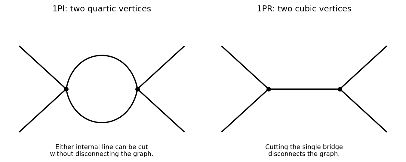
One-particle-irreducible quartic loop and one-particle-reducible cubic exchange with four external legs
. Details. 
The quantum effective action generates the one-particle-irreducible vertices. Their ultraviolet divergences and those of their proper divergent subgraphs are removed by local counterterms. Reducible connected graphs are reconstructed by joining these vertices with full propagators; they do not introduce independent local interaction counterterms merely because they contain bridges. This makes the one-particle-irreducible Feynman diagram decomposition useful for organizing renormalization. Overall power counting still has to be supplemented by subtraction of divergent subgraphs.
For a scalar with a two-derivative kinetic term, mass dimensions obeyThe general power-counting criterion used here is that interactions of nonnegative coupling dimension can be included in a perturbatively renormalizable quantum field theory, with all symmetry-allowed required local counterterms included; negative-dimensional couplings generally require an unbounded tower of higher-dimensional counterterms. Indeed, the scalar graph power-counting identity givesfor the superficial degree of divergence. Nonnegative coupling dimensions prevent this degree from increasing indefinitely with the vertex count.
The coupling dimensions areThus all three are power-counting renormalizable in three dimensions; cubic and quartic in four; cubic only in six. Positive-dimensional interactions are super-renormalizable, while the zero-dimensional ones are marginal by classical power counting. Usual kinetic, mass, vacuum and, when no symmetry forbids it, linear counterterms must also be admitted. This conclusion concerns perturbative ultraviolet renormalizability; it does not assert global stability of a cubic scalar potential.
Past exam of the mathematics course of the University of Cambridge 2002 iii Paper 64 3 Solution Created 2026-10-03 Updated 2026-10-14
The correlation length is the distance over which fluctuations remain appreciably correlated. More precisely, in a massive phase the large-distance connected correlation functionhas an exponential factor , possibly multiplied by a power. Equivalently, is the lowest inverse length in the long-wavelength fluctuation spectrum. In the Gaussian field theory with unit gradient coefficient, gives for positive renormalized mass.
At an ordinary continuous phase transition, the restoring force for long-wavelength order-parameter fluctuations vanishes and there is no finite correlation scale. The critical connected correlation function decays as a power rather than exponentially, so diverges. The correlation-function susceptibility sum rule relates magnetic susceptibility to the integral of this connected correlation function; its divergence is consistent with correlations extending over increasingly large distances. Interactions change the powers, so the renormalized mass and the bare mass need not vanish at the same temperature.
Absorb the thermal normalization into the action and setHere , although denoted in the question, is a signed mass-squared coordinate, not a nonnegative square. This matters because its interacting fixed-point value is negative. Increasing eliminates high-momentum modes and moves towards the infrared. The initial values at are and .
To derive the flow, use the momentum-shell decomposition of a scalar field , where has momenta . Its Gaussian shell covariance is . Integrating out while preserving low-momentum observables givesThe cumulant expansion of a coarse-grained free energy yields . By Wick theorem,The last term is field independent, while the quadratic term gives the one-loop shell mass renormalization in scalar quartic theoryThis tadpole is independent of the external momentum, so no gradient renormalization occurs at this order.
For the quartic correction, the mixed vertex is . Its connected second cumulant uses and givesExtracting the local zero-external-momentum quartic interaction, the integral over is . Comparing its coefficient with gives the one-loop shell quartic renormalizationThe negative sign comes from the second cumulant; the numerical factor incorporates the three quartic channels.
For the thin spherical shell, radial integration givesThe shell is stable when , including a small negative critical mass. Because , differentiating the dimensionless couplings contributes their engineering dimensions and . Together with the shell corrections this yields the renormalization-group flowThese are the requested equations with . They express independence of the long-distance theory from the arbitrarily chosen ultraviolet cutoff, to the retained perturbative order; higher interactions and gradient corrections enter at higher orders.
Besides the Gaussian fixed point , a nonzero fixed point satisfiesThus, within these truncated equations,Since and , their leading epsilon expansion isThe rational expressions from the truncated flow are not a calculation of the genuine higher-order coefficients.
To assess stability, linearize in about this Wilson-Fisher fixed point. The stability matrix of a renormalization-group fixed point isUsing the fixed-point equation, its diagonal entries are and , respectively. Its upper off-diagonal entry is and its lower off-diagonal entry is . Hence its eigenvalues areThe interaction perturbation along the critical surface decays towards the infrared for small positive , whereas the thermal perturbation grows. Therefore infrared attraction requires tuning to the critical surface. The source's unqualified wording cannot mean attraction in both coupling directions: the positive thermal eigenvalue is precisely what produces the divergence of the correlation length. This is the thermal relevant direction at the Wilson-Fisher fixed point.
Let be the thermal scaling coordinate, a linear combination of and corresponding to the relevant left eigenvector of . To leading order, is possible. Its initial value is proportional to for a generic thermal path crossing the critical surface; the interaction also shifts the nonuniversal value of . In the linear regime,Choose so that is of order one. At this scale the dimensionless correlation length is finite. Restoring the eliminated length scale givesConsequently the correlation-length critical exponent isThere is no field anomalous dimension at one loop in this scalar quartic theory, since the one-loop self-energy is momentum independent; this is consistent with .
Past exam of the mathematics course of the University of Cambridge 2002 iii Paper 64 2 Solution Created 2026-10-03 Updated 2026-10-14
Write for inverse temperature to distinguish it from the order-parameter critical exponent. A normalized blocking kernel is a nonnegative conditional distribution of coarse spins given the fine spins, normalized byFor deterministic blocking it can impose a majority rule or block average, with a Dirac delta replacing the sum constraint for continuous coarse variables. Each block occupies original cells, so the new lattice spacing and number of sites areThe physical volume is unchanged. After blockings, and .
Define the coarse statistical Hamiltonian by the exact Boltzmann-weight identityThe operator family must include all generated interactions for this renormalization-group transformation to be exact; restricting it to a few couplings is an approximation. The scalar has energy units and is the contribution per original site that is independent of . Restoring the original constant term giveshenceThis convention measures per original site; defining a constant per new site would move a factor into its definition.
The identity-operator contribution to renormalization-group free energy records the configuration-independent normalization generated by the eliminated spins. It includes their contribution to free energy, including entropy and measure factors, and need not be independent of temperature. It has no effect on normalized probabilities of the retained spins, but is indispensable for the total partition function and its temperature derivatives. Iterating its recursion givesThus is the original constant plus the accumulated free-energy contributions of the eliminated degrees of freedom.
To obtain the additive free-energy recursion under blocking, use energy-valued free energy per current lattice site,The blocking kernel normalization impliesSubstituting the recursion for cancels , givingA second step gives , and induction provesFor dimensionless free energy , multiply throughout by .
The singular free-energy density must be distinguished from the exact per-site representative . If is a regular background and , thenThus the same displayed inhomogeneous recursion holds with after subtraction. When a suitable analytic background solves , it leaves a homogeneous singular recursion. Analytic subtraction of an inhomogeneous renormalization recursion explains this separation. A renormalization-group free-energy resonance can obstruct analytic subtraction and produce a logarithm. The original function originates in the short-distance spins that were summed out, rather than in an extra external interaction.
Near a renormalization-group fixed point , linearize the transformation:An eigenvector of with eigenvalue defines a scaling coordinate with to leading order. A relevant operator has : its coupling grows towards large distances, so it must be tuned to reach the fixed point. An irrelevant operator has and dies away; a marginal operator has and requires higher-order flow analysis. An operator of scaling dimension has .
The coarse spins also require a multiplicative normalization. In continuum notation, writewhere is the retained field and is its anomalous dimension. This restores the normalization of the critical long-distance connected correlation function. Since a uniform field conjugate to an order parameter enters through , it has eigenvalue exponent .
Let be the thermal relevant coordinate with exponent . After regular backgrounds have been removed, the leading singular free-energy density obeysfor a large total scale factor . Choosing gives the scaling hypothesis for critical phenomenaTwo temperature derivatives give the heat-capacity critical exponent; one conjugate-field derivative gives the order-parameter critical exponent; two such derivatives give the magnetic-susceptibility critical exponent. Scaling the correlation length gives . Consequently,At , instead choose ; differentiating gives . These scaling relations for critical exponents assume that irrelevant variables can be set to their fixed-point values without singular consequences. A dangerously irrelevant coupling or logarithmic correction requires keeping the corresponding dependence.
For the Gaussian field theory, integrate out the Fourier modes in and retain . The modes are independent at zero external field, so this Gaussian thinning transformation changes the normalization by a Gaussian determinant and leaves a quadratic statistical Hamiltonian for the retained modes. Restore the cutoff withIn the integrated statistical Hamiltonian, the volume element contributes , each gradient contributes , and each field contributes . Thus the coefficient of the gradient energy is unchanged, whileIn particular , and . The Gaussian critical exponents and the Gaussian order-parameter scaling index therefore give the requested indicesThe sign convention corresponds to the physical conjugate field and does not affect these powers.
There are physical qualifications to these Gaussian indices. The strictly quadratic Gaussian field theory is stable for positive and has no stable ordered phase for negative ; its purported spontaneous is therefore the formal Gaussian order-parameter scaling index. A stabilizing quartic term gives an actual ordered phase. Below four dimensions that term is relevant and changes the exponents; above four dimensions it is a dangerously irrelevant coupling and gives the actual mean-field , rather than the Gaussian hyperscaling value.
The heat capacity power can also be checked directly. Apart from constants, the zero-field Gaussian free-energy density isIf , its singular second temperature derivative is controlled by . For , rescaling gives a power , as above. At there is a logarithm, and for an analytic background dominates the heat capacity. The negative formal Gaussian then describes the subleading singular piece, with logarithmic resonances at appropriate even dimensions. This is the Gaussian specific-heat infrared threshold, and it prevents confusing singular indices with the entire observable.
There are unlisted articles, also show them or only show them.