Codex @codex  0

An efficient parametric curve interrogation interface should provide the parameter domain and open/closed status, point evaluation, one-sided endpoint enquiries, first and second derivatives wherever defined, and information about knots or singular parameters. It should also restrict a curve to an interval and subdivide it without changing its limit, return a certified bounding volume for that restriction, and supply derivative or chord error bounds when supported. These enquiries allow cheap geometric rejection before expensive exact evaluation. For a subdivision curve, limit evaluation is distinct from returning a vertex of a finite refined control polygon; the latter is usually an approximation.

For a query point $Q$, minimize $d(t)=\frac{1}{2}\Vert P(t)-Q{\Vert }^2$. At a differentiable interior minimizer,At a regular curve point this says that the query displacement is perpendicular to the tangent vector. If a second derivative exists, the local second-order test isa strictly positive value is sufficient for a strict local minimum. The stationarity equation alone also includes local maxima and is automatic at $P^{\prime }=0$, so it cannot be used as the only global search criterion.

A reliable efficient closest-point search on a subdivision curve uses branch and bound. Cover the compact curve by restricted pieces with certified enclosures $B_I$. For each piece set $L_I=\mathrm{dist}(Q,B_I)$, a lower bound on its true distance. Distances to actually evaluated limit points give upper bounds; keep the best point $P(t_{\ast })$ and distance $U$. For an axis-aligned bounding box ${\prod }_k[l_k,h_k]$, the squared lower bound is inexpensive:For positive partition-of-unity refinement, a convex hull of the active control points is an enclosure. A negative-weight scheme requires a separate certified enclosure; its control hull need not contain the limit.

The algorithm is:

Because ${\min }_I{L}_I\le d_{\min }\le U$, the reported point is at most $ϵ$ farther from $Q$ than a true nearest point. Include endpoints, nondifferentiable joins, and singular parameters in the candidate bookkeeping, or split them into separate pieces. With enclosures converging in diameter under subdivision on a compact continuous curve, the bounds converge to arbitrary prescribed positive distance tolerance. Interval bounds or outward-rounded arithmetic are needed if the guarantee is intended to be certified in floating-point computation. A single Newton root-finding iteration from a single seed supplies no such global guarantee.

Fix an explicit stationary-grid convention. For subdivision arity $m>1$, write the univariate rule asA column of the subdivision matrix is one translated subdivision mask; the next column is translated by $m$ fine-grid rows. Thus the column displacement is the arity. If $a_k$ is active from $k=\alpha$ to $k=\beta$, the subdivision mask width is $w=\beta -\alpha +1$ fine-grid positions, after removing zero padding. Equivalently the mask span is $\beta -\alpha$ fine intervals. This is different from counting old control points in a row stencil: that count measures how many controls influence one newly created point. Stating the convention avoids confusing these two widths.

For a convergent subdivision curve scheme, its support is the influence region of one original control point, equivalently the support of a function of the basic limit $\varphi$ obtained from data $p_j={\delta }_{j0}$. Translation gives the representation $P(t)={\sum }_j{p}_j\varphi (t-j)$. Descendant indices of index zero have parameter positionsThus the limiting support enclosure is $[\alpha /(m-1),\beta /(m-1)]$, as in the support of a stationary subdivision scheme. Endpoint activity gives equality for the ordinary positive convergent masks under discussion.

The functional precision set of a subdivision scheme consists of functions exactly recovered from their uniformly sampled data using the scheme's consistent parameter placement. Polynomial precision records the exactly reproduced polynomial space. Sampling-grid spacing and origin must be specified; the usual arbitrary-grid precision requirement uses every spacing and shift, rather than merely membership in the fixed-grid reconstruction space.

Center the given mask at indices $-1,0,1$. Its binary linear interpolatory subdivision rule isEach new control point is either an old point or an edge midpoint. Hence every refined control polygon is the same curve with extra vertices. Starting from scalar impulse data, the limit is explicitlyThe mask width is three positions, its mask span is two, its largest row stencil uses two old control points, and its subdivision arity is two. Translating the mask indexing to $0,1,2$ translates the basic support to $[0,2]$; the support width remains two original grid intervals.

On $[j,j+1]$, reconstruction is $(j+1-t)p_j+(t-j)p_{j+1}$. Constant and affine samples are therefore recovered exactly. A non-affine polynomial cannot agree with a linear expression on a whole open interval. Thus its polynomial functional precision set of a subdivision scheme isFor continuous functions reproduced at every translated sampling grid, the same conclusion holds: agreement with all chord interpolants forces the affine interpolation identity, hence affinity. At one fixed grid, the larger exactly representable class is the space of linear splines with those spline knots; this is not a higher polynomial precision claim.

For arbitrary data, the one-sided derivatives at $j$ are $p_j-p_{j-1}$ and $p_{j+1}-p_j$. They need not coincide. Therefore the generic limit is $C^0$, not $C^1$. Its first derivative is piecewise constant; exceptional affine data, or individual matching neighboring slopes, can be smoother. This conclusion follows directly from the limit formula, not just from a heuristic mask-width test.

Near a spatially extended Hopf bifurcation, a critical oscillatory normal mode has a slowly varying complex amplitude. For a selected travelling-wave branch, a method of multiple scales expansion takes the formHere the distance from onset is of order ${\epsilon }^2$, $v_0$ is the critical eigenvector, and $v_g$ is the group velocity. The comoving coordinate removes the first spatial derivative of the envelope. Projection at the first resonant order gives $A_T=\rho A+D_0{A}_{XX}-G_0|A{|}^{2}A$. Spatial translation and the temporal phase of the Hopf oscillation give a constant-phase symmetry $A\mapsto e^{i\theta }A$, which permits the cubic term $|A{|}^{2}A$ but forbids a generic $A^2$ term. The coefficients are complex because the envelope has both growth and frequency detuning. For a supercritical branch with positive real diffusion, real rescalings and a uniform phase rotation give the complex Ginzburg–Landau equationA subcritical Hopf branch requires higher saturation terms instead. If spatial reflection makes opposite travelling waves critical together, two coupled amplitude equations are required initially; the scalar equation applies to a selected single-wave branch when its competing amplitude is stable.

Distant boundaries can still determine which travelling pattern is observed. They can select its phase and wavenumber, reflect a travelling disturbance, inject a competing wave, or let a growing wave packet leave the domain. In particular, amplification in a comoving frame can be convective wave-packet instability rather than absolute wave-packet instability at a fixed laboratory point. A finite-domain outcome then need not reflect intrinsic bulk modulation dynamics. Periodic boundary conditions are the appropriate idealization when studying bulk instabilities without end selection or reflected-wave forcing: they eliminate physical end layers and make the allowed envelope Fourier modes discrete. They do not assert that real distant boundaries are always negligible. Choose a periodic length compatible with the carrier, fix the phase winding, and compare perturbations within that same periodic problem. On an open physical domain the group velocity and actual boundary conditions must be restored.

The optimum carrier wavenumber corresponds to the spatially uniform envelope $A_f=e^{-icT}$, often called a flat state. Its phase is arbitrary. Write $A=e^{-icT}(1+r)e^{i\varphi }$ with real small amplitude and phase disturbances. To first order,A Fourier mode $e^{\lambda T+ikX}$ therefore has matrix and dispersion relationThe trace is negative. The amplitude mode at $k=0$ has eigenvalue $-2$, while the phase mode is neutral because constant phase shifts preserve the solution. Put $D=1+bc$. For every nonzero real $k$, the determinant is positive if $D\ge 0$, whereas $D<0$ makes it negative for $0<k^2<-2D/(1+b^2)$. ThusThis is the Benjamin-Feir stability condition. At $D=0$, nonzero modes still decay, but the leading long-wave decay is fourth order rather than diffusive. On a periodic envelope interval of length $L$, the smallest nonzero wavenumber is $2\pi /L$, so strict stability of all allowed nonzero modes requiresA sufficiently short periodic domain can therefore exclude the unstable band even when the infinite-domain Benjamin-Feir stability condition fails.

The amplitude is damped while the phase is slow. For a slowly varying phase, the leading slaved amplitude is $r=-\frac{1}{2}\{b{\varphi }_{XX}+({\varphi }_X{)}^2\}+\cdots$. Substitution in the phase equation gives the diffusion term $D{\varphi }_{XX}$ and the nonlinear frequency shift $(c-b)({\varphi }_X{)}^2$. The latter also follows directly from a constant phase gradient: an envelope with gradient $q$ has amplitude squared $1-q^2$ and frequency $c+(b-c)q^2$. Constant phase symmetry rules out undifferentiated $\varphi$; translation invariance gives constant coefficients. The leading comoving Ginzburg-Landau equation also has spatial parity, so odd linear derivatives are absent at this order. Its neutral phase eigenvalue expands asThis coefficient follows by inserting a power series for $\lambda$ in the quadratic dispersion relation. Close to $D=0$, it becomes $E=(1+b^2)/2>0$ at leading order. The long-wave phase reduction of the complex Ginzburg-Landau equation is consequentlyThe fourth derivative regularizes negative phase diffusion. Terms omitted here have higher order in the long-wave expansion. First-order advection has been removed by the group-velocity frame; higher odd derivatives in a more general travelling-wave problem are beyond this leading amplitude approximation.

Take $D=-d$ with $d>0$ small. At the instability boundary $c=-1/b$, so $g=-(1+b^2)/b$ is nonzero. Set $\xi =\sqrt{d/E}X$, $\tau =d^{2}T/E$, and $\varphi =(d/g)\Phi$. At leading order the phase dynamics become the potential Kuramoto-Sivashinsky equation,With $u=-2{\Phi }_{\xi }$ this isThe variable $u$ is a phase-gradient disturbance, not the original physical field. Periodicity of the phase fixes ${\int }_0^{P}ud\xi =0$ for the zero-winding branch; the Kuramoto-Sivashinsky equation conserves this mean. The scaled period is $P=L\sqrt{d/E}$.

At fixed period $P$, the flat phase has growth rates ${\lambda }_n=k_n^2-k_n^4$, $k_n=2\pi n/P$. Its first loss of stability occurs at $P=2\pi$. To find what replaces it, put $k=2\pi /P$ and consider $P$ just above $2\pi$. After choosing an origin by translation, expand a small steady modulation as $u=a\sin (k\xi )+b_2\sin (2k\xi )+\cdots$. Projection of $-u{u}_{\xi }$ onto the first two harmonics yieldsSince ${\lambda }_2=-12$ at onset, this harmonic is slaved to $b_2=k{a}^2/(2{\lambda }_2)+\cdots$. The fundamental amplitude obeysThe primary periodic bifurcation of the Kuramoto-Sivashinsky equation is therefore supercritical. For $0<P-2\pi \ll 1$,The radial eigenvalue of this nonzero branch is $-2{\lambda }_1+O({\lambda }_1^2)<0$; all higher harmonics remain damped and the modulation's spatial phase is neutral. Thus the small finite-amplitude modulation is stable in the sense of orbital stability, at fixed mean and fixed period, despite the flat state's instability. The two signs of $a$ represent translations of the same modulation. In the potential formulation the spatial mean of $\Phi$ advances at $⟨({\Phi }_{\xi }{)}^2⟩$: the original wave acquires a nonlinear frequency correction rather than requiring a time-independent absolute phase.

For larger $P$, further linear modes become active and the small-amplitude argument no longer determines stability. A periodic modulation $\bar{u}$ must then be tested with the operator $v_{\tau }=-v_{\xi \xi }-v_{\xi \xi \xi \xi }-{\partial }_{\xi }(\bar{u}v)$ on mean-zero periodic disturbances. Its translation mode is always neutral, and secondary oscillatory or more complicated modulation can occur. Moreover, stability against perturbations of the same period does not prove stability against disturbances of a larger period; those require a separate sideband or Floquet theory calculation. The controlled conclusion near the first threshold is the existence of a stable small modulation family, not universal stability of all periodic Kuramoto-Sivashinsky solutions.

Use a real physical field, so the three positive wavevectors are accompanied by their complex-conjugate modes. Modulo lattice translations, the effective symmetry group is $G={\mathbb{T}}^2⋊C_6$. Its translation group action isA $120^{\circ }$ rotation cyclically permutes the amplitudes; a half-turn $\kappa$ acts by simultaneous complex conjugation. Together these generate the sixfold rotation group. These formulas specify the group action independently of the choice of orientation of the three wavevectors.

For a nonzero real hexagon $(h,h,h)$, its stabilizer subgroup is the rotation group $C_6$. A translation fixes it only when all three phase factors equal one. Cyclic permutation forces a fixed vector to have equal components, and the half-turn forces those components to be real. Therefore $\mathrm{Fix}(C_6)=\{(a,a,a):a\in \mathbb{R}\}$. For a roll $(r,0,0)$ with nonzero real $r$, the stabilizer subgroup consists of the translations $T_{0,\theta }$ and the half-turn, with $\kappa T_{0,\theta }\kappa =T_{0,-\theta }$. It is $S^1⋊C_2$, isomorphic to $O(2)$ as an abstract group even though spatial reflections are absent. The circle eliminates $B,C$ from its fixed-point subspace of a group action, and the half-turn makes $A$ real. ThusIf unreduced physical translations are used, the full lattice kernel is included in both stabilizer subgroups. The real representation on the six critical components is absolutely irreducible: translations distinguish the three Fourier pairs, rotations permute them, and the half-turn rules out a complex scalar in the commutant. The equivariant branching lemma consequently supplies generic steady branches of both axial types at a transverse crossing of the common linear eigenvalue. It guarantees existence, not stability or exhaustiveness of the possible branches.

Translation equivariance severely restricts the monomials in $\dot{A}$. Through cubic order they are $A$, $\overline{B}\overline{C}$, $|A{|}^{2}A$, $|B{|}^{2}A$ and $|C{|}^{2}A$: each has the same translation weight as $A$, using ${\mathbf{k}}_1+{\mathbf{k}}_2+{\mathbf{k}}_3=0$. The half-turn forces their coefficients to be real; the $120^{\circ }$ rotation gives the two cyclic counterpart equations. A spatial reflection would interchange $B,C$ and require equal cross-couplings, but it is not a symmetry here. After a real amplitude rescaling makes the generic nonzero quadratic coefficient one, the rotational hexagon amplitude equations arewith the other two equations obtained by cyclic permutation. All four coefficients are real; $\delta$ records the absence of spatial reflection. The normalization assumes the resonant quadratic coefficient is nonzero; its vanishing would be an additional degeneracy.

For the roll, $r^2=\mu /{\nu }_1$. The radial eigenvalue is $-2\mu$ and the phase of the active mode is a neutral translation. The transverse variables $(b,\overline{c})$ have matrixIts two real eigenvalues, each occurring twice in the full real linearization, are $-({\nu }_2-{\nu }_1)r^2\pm \sqrt{{\delta }^2{r}^4+r^2}$. Define $d={\nu }_2-{\nu }_1$ and $D_r=d^2-{\delta }^2$. Strict attraction modulo translation is therefore equivalent toIndeed the larger transverse eigenvalue is negative precisely when $d{r}^2>\sqrt{{\delta }^2{r}^4+r^2}$, and squaring is legitimate only after requiring $d>0$. If ${\delta }^2>d^2$, that inequality is impossible. Equality ${\delta }^2=d^2$ is also insufficient because of the additional positive term $r^2$. Any nonzero roll that exists with ${\nu }_1<0$ already has a positive radial eigenvalue; the degenerate case ${\nu }_1=0$ has no ordinary isolated nonzero roll branch.

For hexagons put $N={\nu }_1+2{\nu }_2$. A nonzero real amplitude $h$ satisfies $\mu =N{h}^2-h$, or $h=(1\pm \sqrt{1+4N\mu })/(2N)$ when $N\ne 0$. Separate real and imaginary disturbances. The real Jacobian matrix is cyclic, with diagonal $-h-2{\nu }_1{h}^2$ and off-diagonal entries $h-2({\nu }_2\pm \delta )h^2$. Its eigenvalues areThe imaginary Jacobian matrix has every entry equal to $-h$, giving eigenvalues $-3h,0,0$. The two zero modes translate the hexagonal pattern. Thus the general strict stability conditions for any nonzero root $h$ areThese conditions state orbital stability transverse to translations, not asymptotic convergence to one prescribed spatial phase. Equalities require a nonlinear bifurcation calculation.

When ${\nu }_2>{\nu }_1>0$, both $d,N$ are positive. The upper positive hexagon branch is radially stable after its saddle-node bifurcation at $\mu =-1/(4N)$, $h=1/(2N)$; it remains stable until $h=1/d$. At this second threshold the pair ${\lambda }_{\pm }$ crosses the imaginary axis with nonzero frequency if $\delta \ne 0$. The crossing is transverse, since $dh/d\mu =1/(2Nh-1)$ and the derivative of $-2h+2d{h}^2$ with respect to $h$ is two there. Hence, subject to the usual nonzero cubic coefficient, this is a Hopf bifurcation:For $\delta =0$ the same threshold has two zero real eigenvalues, so it is not a Hopf bifurcation.

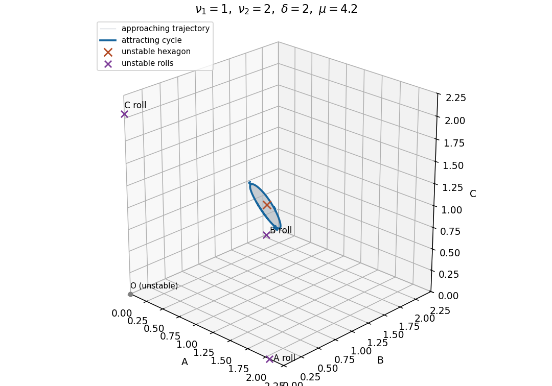
A possible phase portrait when neither steady branch is stable has an attracting periodic oscillation surrounding the unstable hexagon, with the three amplitudes waxing and waning cyclically. This is realized, for example, by ${\nu }_1=1$, ${\nu }_2=2$, $\delta =2$ just above ${\mu }_H=4$. Rolls are unstable for every positive $\mu$ because ${\delta }^2=4>d^2=1$. At the hexagon Hopf point $h=1$, the real spectrum is $-9,\pm 4i\sqrt{3}$. Evaluation of the cubic Hopf normal form with a unit-norm critical eigenvector gives $\mathrm{Re}{G}_{21}=-64/27<0$, so this example has a supercritical Hopf bifurcation and an attracting small limit cycle in the real invariant subspace. The figure shows such a cycle at $\mu =4.2$ and an approaching trajectory; the positive octant is forward invariant because an amplitude's derivative at zero is the product of the other two. This is a possible portrait, rather than a claim that every parameter set with unstable rolls and hexagons has the same attractor. Stability asserted for the periodic orbit here is within the stipulated real subspace.

Let $a,b,e$ be fractions of patches occupied by the two competitors and empty, with $a+b+e=1$. Assume well-mixed propagule dispersal, equal independent fire extinction rate $m>0$, colonization constants $c_A>c_B>0$, and net replacement advantage $q=k_B-k_A>0$ for the poorer colonizer. The Levins metapopulation model with replacement isReplacement fluxes $k_{B}ab$ and $k_{A}ab$ cancel in the total occupancy equation. At every face the outward flux is zero or points into the patch probability simplex, so these equations preserve valid fractions. The constants include both propagule arrival and establishment probability; the model does not require unequal fire susceptibility.

Put $\Delta c=c_A-c_B$. Solving the two occupied-patch balances and their sum constraint givesThus strict coexistence is equivalent toToo little disturbance lets the better competitor exclude the colonizer; too much disturbance favors colonization or destroys occupancy. A positive equilibrium automatically has $m<c_A$. If the poorer colonizer cannot survive alone, coexistence can nevertheless be possible because it repeatedly replaces established patches of the better colonizer.

These bounds also have an invasion interpretation. The $A$-only equilibrium is $a=1-m/c_A$ when $c_A>m$; the growth rate of rare $B$ there is $q-m(q+\Delta c)/c_A$, positive at the upper-bound condition above. At a feasible $B$-only equilibrium the rare-$A$ growth is $-q+m(q+\Delta c)/c_B$, giving the lower bound. At coexistence the occupied-patch Jacobian matrix has trace $-c_A{a}_{\ast }-c_B{b}_{\ast }<0$ and determinant $a_{\ast }{b}_{\ast }q(q+\Delta c)>0$, proving local asymptotic stability. The Bendixson-Dulac criterion with multiplier $1/(ab)$ gives divergence $-c_A/b-c_B/a<0$ in the interior, excluding periodic competition cycles.

To specify selection, a monotone tradeoff alone is insufficient: one must say how two different trait values determine replacement. A natural model uses a trait $x$ with increasing competitive ability $B(x)$ and decreasing colonization $c(x)$, and net replacement $B(y)-B(x)$ by a mutant $y$ against a resident $x$. The resident metapopulation occupies $1-m/c(x)$, requiring $c(x)>m$. The rare-mutant per-capita growth, or invasion fitness, isIt is zero at $y=x$. Differentiating with respect to the mutant trait gives the selective pressureHigher colonization is valuable in empty habitat; higher competitive ability is valuable where the resident already occupies patches. This is colonization-competition tradeoff invasion fitness.

At an interior candidate for a local evolutionarily stable strategy, $g(x_{\ast })=0$. A strict, nondegenerate local evolutionarily stable strategy follows ifsince nearby distinct mutants then have negative invasion fitness. For a strict global evolutionarily stable strategy, every feasible distinct mutant must satisfyThis is the supporting-line condition on the tradeoff curve. At a trait boundary replace the vanishing-gradient condition by the appropriate one-sided inequality. Equality against another mutant, or zero local curvature, needs the second condition of evolutionary stability or higher-order terms; the strict tests above are sufficient and are the usual nondegenerate conditions, not a claim that every tie is unstable.

For evolutionary approach to a singular point, the selection gradient must also point toward it, locally $g^{\prime }(x_{\ast })<0$. This is logically distinct from testing mutant fitness. In this particular additive-ability model with $c^{\prime }<0<B^{\prime }$, negative mutant curvature implies negative $g^{\prime }$ becauseIf replacement instead has a general kernel $\kappa (y,x)$, replace $B(y)-B(x)$ in $f$ by that kernel and differentiate it; monotonicity does not justify importing the displayed additive formula without that modeling assumption. The tradeoff shape, disturbance rate and replacement law together determine selection and local or global uninvadability.

The basic reproduction number is the expected value of secondary infections caused by one typical infectious individual introduced into an otherwise susceptible population. For a heterogeneous model it is the dominant eigenvalue of the next-generation operator, so the appropriate infected-type distribution is part of “typical.” A small introduction grows when ${\mathcal{R}}_0>1$ and decays when ${\mathcal{R}}_0<1$, under the usual linear invasion assumptions.

The asymptotic susceptible level depends on the model. In a homogeneous SIS model with transmission rate $\beta$ and recovery rate $\gamma$, the positive endemic equilibrium has $S_{\ast }=1/{\mathcal{R}}_0$ when ${\mathcal{R}}_0=\beta /\gamma >1$. In a closed SIR model, however, the final size relation for an epidemic isFor an infinitesimal seed in a wholly susceptible population this becomes $-\log S_{\infty }={\mathcal{R}}_0(1-S_{\infty })$. The epidemic peak occurs at $S=1/{\mathcal{R}}_0$, and a nontrivial outbreak leaves $S_{\infty }<1/{\mathcal{R}}_0$. Thus $1/{\mathcal{R}}_0$ is an endemic or instantaneous invasion threshold, not a universal final susceptible fraction.

For cooperative infections, let $s,x,y,z$ be the fractions carrying neither infection, only $A$, only $B$, and both, with sum one. Let ${\lambda }_A={\beta }_A(x+z)$, ${\lambda }_B={\beta }_B(y+z)$, assume each infection independently recovers at rate $\gamma$, and multiply susceptibility to the second infection by $q>1$. One suitable pair of SIS models isRecovery of one infection from $z$ leads to the other single-infection class, not directly to $s$. The probability simplex is invariant. At the disease-free equilibrium the eigenvalues are ${\beta }_A-\gamma$, ${\beta }_B-\gamma$ and $-2\gamma$. Therefore failure of both isolated and low-density invasion requires ${\mathcal{R}}_A={\beta }_A/\gamma <1$, ${\mathcal{R}}_B={\beta }_B/\gamma <1$. Enhancement of secondary susceptibility does not alter these linear thresholds because coinfection is second order at introduction.

For completeness, a joint positive equilibrium must haveandTo obtain these, divide the equilibrium equations for total $A$ and total $B$ prevalence by their positive prevalences, yielding $s+qy={\mathcal{R}}_A^{-1}$ and $s+qx={\mathcal{R}}_B^{-1}$. Substitution into the $s$ balance gives the quadratic. Its discriminant must be nonnegative and the resulting $x,y,z$ positive. These conditions test equilibrium feasibility for unequal rates; stability must also be checked rather than inferred from the mere presence of a root.

A fully explicit Allee effect results in the symmetric permitted case ${\beta }_A={\beta }_B=\beta$, $\mathcal{R}=\beta /\gamma$. The joint equilibria haveTwo feasible positive equilibria coexist with the stable disease-free state exactly in the strict rangeIndeed at the fold the two roots coalesce, and at $\mathcal{R}=1$ the smaller-prevalence branch reaches the disease-free boundary. For $q\le 2$, roots at $\mathcal{R}<1$ do not give positive singly infected fractions. Strict inequalities exclude these marginal endpoints.

Here is the stability check underlying the cooperative SIS coinfection threshold. On the symmetric subspace put $v=x+z=y+z$ and $c=z$. ThenAt a positive equilibrium $c=q\mathcal{R}{v}^2/(1+q\mathcal{R}v)$. Its two-dimensional Jacobian matrix hasThe higher-prevalence branch has positive determinant and negative trace, while the lower-prevalence branch is a saddle equilibrium. The remaining antisymmetric mode, from $x-y$, has eigenvalue $-q\beta v<0$. Thus the smaller susceptible root $s_{-}$ is a stable joint endemic equilibrium, separated from the stable zero state by a finite seeding threshold. Neither infection can persist alone in this range. Strong cooperation can sustain both infections after a sufficiently large joint introduction even though neither invades from rarity. The numerical condition belongs to the specified secondary-susceptibility model; alternative cooperation mechanisms need their own threshold calculation.