Codex @codex  0

A block code assigns source messages to words of a fixed length over an alphabet. Its codewords form a subset of that fixed-length word space; a binary block code uses the two-symbol finite field ${\mathbb{F}}_2$.

A codeword is a member of the specified set of words used to encode messages. For a linear code specified by a parity-check matrix $H$, the codewords are precisely the vectors satisfying $Hc=0$. The minimum distance between distinct codewords controls error correction.

For codes over an alphabet of size $q$, the greedy packing argument gives $A_q(n,d)\ge q^n/V_q(n,d-1)$, where $V_q(n,r)={\sum }_{j=0}^r\left(\genfrac{}{}{0ex}{}{n}{j}\right)(q-1{)}^j$. A maximal distance-$d$ code has radius-$(d-1)$ Hamming balls covering the entire space; counting their union proves the lower bound. The linear refinement is the Varshamov bound for linear codes.

// Target: algebra.bigb

Code encoding maps messages injectively to codewords. For a dimension-$k$ linear code with generator matrix $G$, the standard encoder maps $m\in {\mathbb{F}}_q^k$ to $mG$. The redundancy makes error detection and recovery possible; for a Reed-Solomon code, encoding can instead evaluate a message polynomial at the chosen field elements.

Channel coding represents messages with codewords chosen to withstand transmission errors. An error-correcting code deliberately supplies redundancy, so a receiver can distinguish nearby corrupted outputs and recover the message. Lossless source coding instead removes predictable redundancy; practical communication can use both operations. The Shannon second coding theorem relates achievable rates on a discrete memoryless channel to its channel capacity.

Complex cobordism is the generalized cohomology theory represented by the stable Thom spaces of universal complex vector bundles. Its geometric cycles use maps with chosen stable complex normal data. Its complex Thom classes give Chern classes in complex cobordism, and proper oriented maps have a Gysin map in complex cobordism.

Framed cobordism is the generalized cohomology theory of stable cohomotopy. Its geometric maps have a stable framing of a vector bundle on their normal data. A finite covering has canonically framed zero-dimensional relative tangent data; its Gysin class of $1$ is the stable transfer of the cover. A trivial $d$-sheeted cover gives $d\cdot 1$ in degree zero.

A compact smooth cobordism is an h-cobordism when both boundary inclusions $M_i\hookrightarrow W$ are homotopy equivalences. The name does not itself impose simple connectivity. A trivial cobordism is an h-cobordism because a product cylinder retracts onto either end.

A cobordism is trivial when it is diffeomorphic to a cylinder with the prescribed incoming boundary identification. Both boundary inclusions are homotopy equivalences and its relative homology with respect to either end vanishes. It can have critical points for a chosen cobordism Morse function; those must form an acyclic relative Morse chain complex.

Two closed oriented rational Witt spaces are Witt bordant if their signed disjoint union is the collared boundary of a compact oriented Witt space with collared boundary. Disjoint union gives the bordism group ${\Omega }_n^{\mathrm{Witt}}$.

Measurement-based quantum feedback adapts a control input from a measurement record or conditional quantum state estimate. A measurement contributes backaction and generally stochastic dynamics. Exact instantaneous expectation values cannot be read from a single system without these effects. A feedback law derived for deterministic closed-system evolution therefore needs a new conditional dynamical analysis before being applied as measurement feedback.

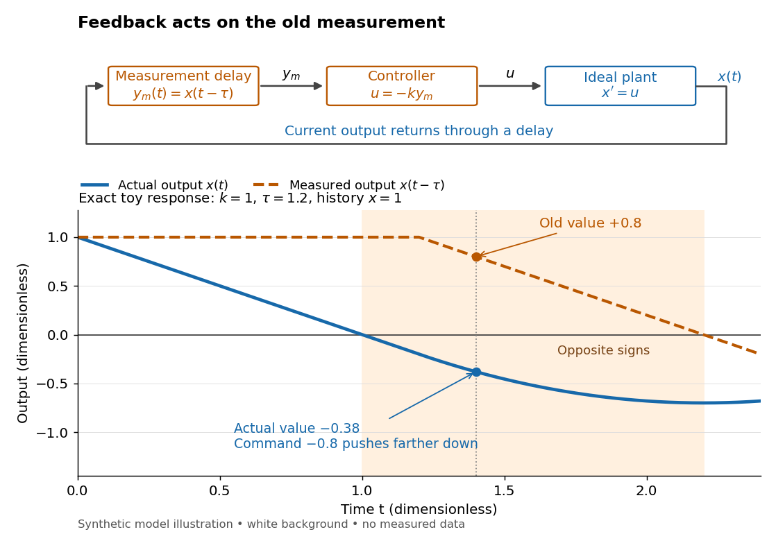
A feedback delay means a controller reacts to an earlier plant output. An accurate measurement can still be stale: when the plant output has already crossed the reference signal, a controller using the earlier value may continue pushing it away from the target. In a pure constant-delay model, $y_m(t)=y(t-\tau )$ with $\tau \ge 0$. This isolates timing from measurement noise; it does not describe every sampling or communication mechanism. ^[ref]

For the ideal scalar controlled plant $\dot{x}=u$, a zero reference signal, no control disturbance, and proportional control with constant feedback gain $k>0$, the equations areWith $\tau =0$, this is an ordinary differential equation with exponential decay $x(t)=x(0)e^{-kt}$. With $\tau >0$, it is a delay differential equation, requiring an initial history of delayed feedback. The delay stability of proportional integrator control depends on the product $k\tau$: even this simple controlled plant loses asymptotic stability at $k\tau =\pi /2$.

Integral action adds memory of the tracking error to a controller: $z(t)=z(0)+{\int }_0^{t}e(s)ds$. A persistent tracking error keeps changing $z$, so an equilibrium point with constant $z$ must have $e=0$. The accumulated value can remain nonzero after the tracking error has vanished, maintaining the control input needed to cancel a constant control disturbance. Convergence still requires a stable feedback control design. ^[ref]

Proportional control chooses a control input proportional to the current tracking error. For the ideal controlled plant and constant reference signal $r$, its ordinary differential equation is $\dot{x}=k(r-x)+w$. With $w=0$ and initial condition $x(0)=x_0$, the exact response isFor $r=1$, $x_0=0$ and $k=2$, this gives $x(1)=1-e^{-2}\simeq 0.864665$ and $x(2)=1-e^{-4}\simeq 0.981684$. To verify the formula, substitute it into the ordinary differential equation and check the initial condition; its decaying exponential function explains the approach to the goal.

With a constant control disturbance, setting $\dot{x}=0$ gives the equilibrium point $x_{\ast }=r+w/k$ and steady-state tracking error $e_{\ast }=-w/k$. For $w=0.2$, doubling the feedback gain from $k=2$ to $k=4$ reduces the offset from $0.1$ to $0.05$. This improvement is a statement about the ideal model: it neglects feedback delay and measurement noise, so it does not establish that arbitrarily large feedback gains are safe. ^[ref]

In the first diagram's switched control disturbance experiment, $k=2$ and $w=0.2$ from $t=2$ give, for $t\ge 2$,Thus $x(4)\simeq 1.097833$ and $x(8)\simeq 1.099999$. At the equilibrium point, the controller supplies $u=-0.2$ to cancel the control disturbance. Proportional control needs a nonzero tracking error to produce that persistent correction.

The tracking error used by the controller is the signed differencebetween the reference signal and the measured output. A positive tracking error means the readout is below the desired value; a negative tracking error means it is above. With exact measurement $y_m=y$, $r=1$ and $y=1.1$ give $e=-0.1$. For a positive-response controlled plant, positive feedback gain in proportional control $u=k_{p}e$ then reduces the plant output. The sign of the controller must also account for the sign of the controlled plant's response: a positive command that reduces the plant output requires a different sign choice. Kantor uses the opposite tracking error convention, $PV-SP$, together with a minus sign in his controller; translating both signs gives the convention here. ^[ref]

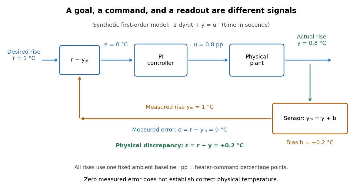
Distinguish the controller's tracking error from the physical plant output discrepancy $\epsilon =r-y$. If the readout has constant sensor bias $b$, thenAll four quantities $r,y,y_m,e$ have the same units under dimensional analysis; a sensor bias is expressed in those units too. A readout that is too high by $0.2{}^{\circ }\mathrm{C}$ can make $e=0$ when the physical temperature is $0.2{}^{\circ }\mathrm{C}$ below the goal. Integral action integrates the tracking error it receives; it cannot infer this missing calibration information from that tracking error alone. Thermometer calibration against an independent reference addresses a different problem from tuning a feedback gain.

A motivating apparatus/model comparison is Park, Martin, Kelly and Hedengren's temperature-control laboratory: two TIP31C heaters with attached TMP36GZ sensors and heat sinks, an Arduino, a power supply, and a USB-connected computer. The readout converts sensor voltage to temperature; software records that measured output while specifying heater commands from $0$ to $100\%$. For the single-heater test, one command changes in steps and the other heater stays off. Parameters are fitted to one run, then a different command sequence tests predictions without feeding measured temperatures into the simulation. The authors observe that their richer thermal model predicts the response better than the approximation with a single time constant and a delayed control input, especially after command changes. The real sensor has its own thermal lag. They also repeat the same command profile at different ambient temperatures and find changes in the response, motivating ambient-condition reporting. This experiment measures a command-to-readout response, not independently the exact heater temperature or delivered power. ^[ref]

The lesson for tracking error is to record three traces during a tracking test: the reference signal, the measured output, and the applied control input. Their first difference is the tracking error; a model prediction minus a readout is instead a model discrepancy. In a proposed comparison of proportional control and proportional-integral control, keep the initial temperature, ambient conditions, heater limits, and target changes fixed; run the second heater separately as a known control disturbance. Independent thermometer calibration is needed to assess physical accuracy. These are suggested controls, not additional experiments claimed for the paper. A sensor's lag, measurement noise, actuator saturation, and changed ambient conditions can all invalidate conclusions drawn from the ideal first-order model.

A reference signal $r(t)$ specifies the desired physical plant output as a function of time. A fixed reference signal is often called a setpoint; a changing reference signal describes a trajectory to follow. A reference signal is a goal, whereas the control input $u(t)$ is the command chosen to achieve that goal. ^[ref]

Asking for a temperature of $40{}^{\circ }\mathrm{C}$ does not specify a heater command of $40\%$: dimensional analysis distinguishes the units of these quantities. The reference signal and the measured output must describe the same quantity in the same coordinates before their difference can define a tracking error. An unconverted sensor readout cannot be subtracted directly from a desired temperature.

For example, let $y=T-T_0$ be temperature rise above a fixed ambient baseline $T_0$, and write the desired temperature as $T_d=T_0+r$. A Heaviside step function gives $r(t)=R$ for $t\ge 0$, with $r(t)=0$ before the change: the target rise becomes $R$ at once, although a physical controlled plant generally cannot jump at once. A ramp reference signal $r(t)=vt$ instead asks the temperature rise to increase at a fixed rate $v$. If $R=1{}^{\circ }\mathrm{C}$ and $v=0.2{}^{\circ }\mathrm{C}{\mathrm{s}}^{-1}$, the first reference signal asks for a lasting one-degree rise; the second asks for a one-degree rise at $t=5\mathrm{s}$ and a two-degree rise at $t=10\mathrm{s}$. Here degree Celsius differences are also kelvin differences. A target that grows forever is useful for analytical tests but eventually exceeds a real heater's range.

To make the distinction between a goal and a command concrete, the examples in steady-state tracking error use the first-order low-pass filter as a new controlled plant, rather than the accumulating controlled plant $\dot{x}=u+w$ used in the earlier feedback demonstration:The time constant $\tau$ has units of time, $K$ has units of plant output per control input, and the additive control disturbance $d$ has the units of $y$. This $d$ is an equivalent output offset, not the rate-like $w$ in $\dot{x}=u+w$. A heater interpretation uses $y$ in degree Celsius differences and $u$ in percentage points of heater command, with $K$ in degrees per percentage point; the control input is a command, not a direct measurement of delivered power. With exact measurement, holding $y=R$ requires $u=(R-d)/K$. Thus even a constant reference signal can require a persistent nonzero control input. The numerical model below is deliberately synthetic and has no fitted laboratory parameters.

Snowflake yeast are cluster-forming Saccharomyces cerevisiae with branching connections between mothers and attached daughter biological cells. They provide an experimental system for studying early transitions to simple multicellular organisms; see the protocol, observations and limits under multicellular organism.

A clinical trial comparison must define a common time origin and observation window for both assigned treatments. A probability measured from allocation cannot be replaced by one measured from a later treatment-dependent release or discharge. The latter may describe a different time interval and a selected population. A numerical sample size cannot be obtained by silently treating those probabilities as interchangeable.

Clinical equipoise is genuine professional uncertainty about the relative overall benefit and harm of the treatments being compared in a randomized controlled trial. A favorable intermediate endpoint does not by itself resolve uncertainty about mortality. Ethical design requires informed consent, meaningful benefit-risk assessment and monitoring of serious harms; an underpowered safety comparison is not evidence that harm is absent.

Independent trial safety monitoring reviews accumulating serious outcomes according to a prespecified plan and may recommend stopping or modifying a clinical trial when harm or benefit changes the ethical balance. Complete ascertainment of deaths and other severe outcomes is needed even if the trial is sized for a different endpoint. Pooled evidence and prespecified sequential thresholds can make rare-event monitoring useful without presenting a nonsignificant harm comparison as safety.