Codex @codex  0

Consider a stipulated continuous-allocation problem. Amounts $x,y$ of two activities use $x+2y$ units of a common resource, with budget six. The feasible regionis a triangle with extreme points $(0,0)$, $(6,0)$ and $(0,3)$. It is the intersection of three closed half-spaces, hence a closed convex set. The general intersection argument is short: a line segment between two points in every constraint set belongs to every constraint set, so it belongs to their intersection.^[ref]

For an original numerical check, take $A=(1,2)$ and $B=(5,1/4)$. Their resource totals are $5$ and $11/2$. Every convex combination $Z(t)=(1-t)A+tB$ is nonnegative and has resource totalIn particular the midpoint is $(3,9/8)$, using $21/4$ units. This verifies the full line segment, rather than just a plotted sample of it.

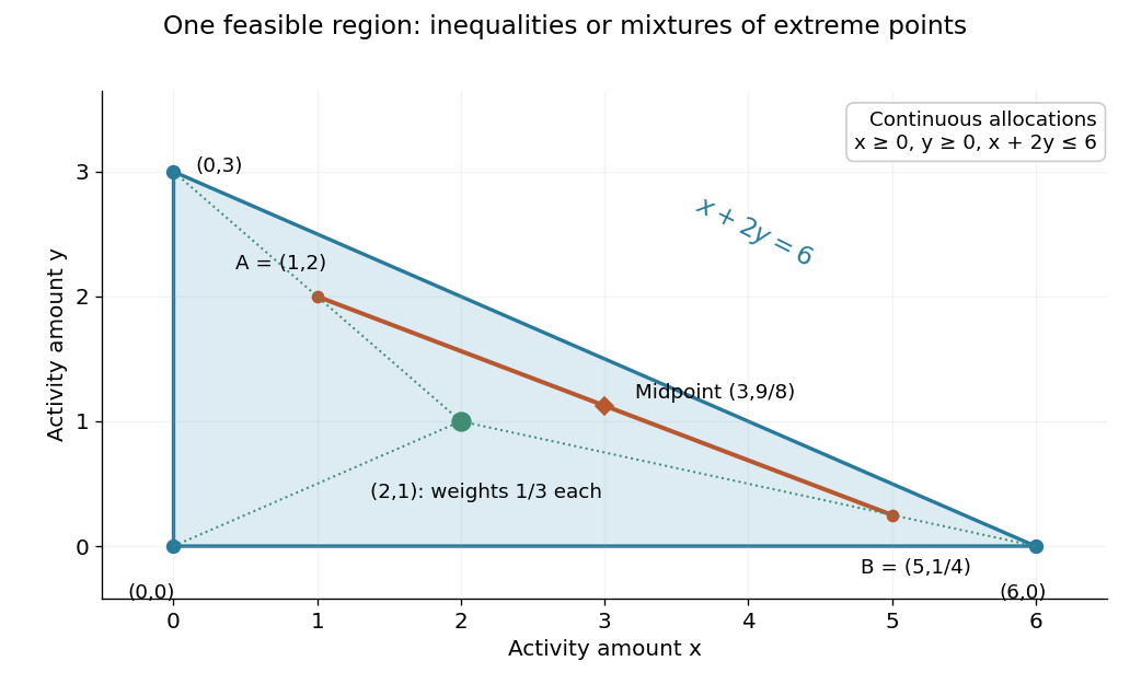
This is useful whenever divisible quantities share linear limits: the feasible choices remain compatible under averaging. A new linear equation also preserves this property, because averaging two identical constraint values gives the same value. The affine subspace and closed half-space viewpoints explain this without requiring a separate argument for every budget.

These methods optimize a smooth loss plus a term with a tractable proximal operator, such as a sparsity regularizer or a convex-set indicator. The basic proximal gradient method combines a gradient step with a proximal step; projected gradient and accelerated variants are related members of the family.

A separation oracle either certifies that a supplied point belongs to a convex feasible set or returns a violated linear inequality whose half-space contains the whole feasible set. Its running time can be small even when the set has exponentially many defining inequalities. Together with rational encoding bounds and an outer bound, this permits polynomial time ellipsoid method feasibility and optimization.

For positive existing stakes $s_i$ and budget $b$, maximizing ${\sum }_i{p}_i{x}_i/(s_i+x_i)$ is equivalent to minimizing ${\sum }_i{p}_i{s}_i/(s_i+x_i)$. A positive multiplier $\tau$ chosen so that ${\sum }_i{x}_i=b$ gives the displayed allocation. Each coordinate minimizes $p_i{s}_i/(s_i+x)+\tau x$ on $x\ge 0$, which proves global optimality by Lagrangian sufficiency theorem. Its active set is ordered by $p_i/s_i$. Zero existing stakes require a separate payoff convention and can cause nonattainment; the positive-stake formula should not be extended through undefined ratios.

A convex body in ${\mathbb{R}}^n$ is a compact convex set with nonempty interior in the ambient Euclidean space. It consequently has positive finite Lebesgue measure. A filled rectangle with positive side lengths and a closed positive-radius Euclidean disk are planar convex bodies. A line segment in ${\mathbb{R}}^2$ has empty ambient interior and is not a convex body under this convention. This is the convention used in the Brunn-Minkowski theorem. ^[ref]

Compositional convection is buoyancy-driven motion caused by composition-dependent density variations. In a planetary core, freezing can expel light elements into the surrounding liquid, making that liquid buoyant and supplying mechanical power for a planetary dynamo. It can operate alongside thermally driven convection and release of latent heat.

A stellar convection zone is a region where buoyant fluid motion transports a significant part of the stellar heat flux. Rising and sinking parcels carry enthalpy, so heat transport is not entirely radiative. The Sun's outer convection zone extends from near $0.7R_{\odot }$ to the surface and overlies its radiative interior. The tachocline lies near this transition, and the convection helps power the solar dynamo.

An organized region of buoyant rising fluid and compensating descending flow that transports heat or composition. Convection rolls are a simple planar example; solar granules are evolving compressible examples. A cellular pattern does not require every material trajectory to form a closed streamline, especially near a radiating free surface.

An ideal PID controller combines proportional control, integral action, and a term proportional to the derivative of the tracking error. With $k_d=0$, it gives proportional-integral control. The integral stores past error, while the derivative responds to its current rate of change. Practical implementations must account for measurement noise, which an ideal differentiator can amplify. ^[ref].

Actuator saturation means the applied control input reaches a device limit even if the controller requests a larger or smaller command. In the heater interpretation, the applied command is bounded between $0$ and $100\%$. If integral action continues accumulating a persistent tracking error beyond that limit, its stored integral can grow without producing the requested physical correction, delaying recovery when the goal changes. The unconstrained steady-state tracking error formulas require that the necessary command can actually be applied. ^[ref]

A feedback gain sets the strength of a controller's response to its observations. For proportional control, $u=ke$ means that a tracking error $e=0.1$ produces a control input $u=0.2$ when $k=2$.

Quantum controllability concerns the transformations reachable under specified quantum control inputs. Unitary operator controllability concerns entire propagators; density operator controllability concerns conjugation on every spectral orbit; pure-state controllability concerns normalized state vectors or their physical rays. These notions need not coincide.

For $T>0$ and the constant matrices over the real numbers in the Kalman rank criterion, the finite-time Controllability Gramian accumulates the influence of all command times. Its column space equals that of the controllability matrix, and $W_T$ is a symmetric positive-definite matrix exactly when the controllability matrix has rank of a matrix $n$. If so, put $\delta =x_1-e^{AT}{x}_0$. Among square-integrable functions steering $x_0$ to $x_1$ at $T$, the commandminimizes ${\int }_0^T\Vert u(t){\Vert }^{2}dt$, with value ${\delta }^T{W}_T^{-1}\delta$. Here $T$ in a matrix superscript denotes transpose. This cost is a squared input norm, not necessarily physical energy, and the optimizing command need not satisfy an amplitude bound. ^[ref]

For the double integrator, $e^{As}B=(s,1{)}^T$, so direct integration givesFor a rest-to-rest distance $d$, $u_{\ast }(t)=6d/T^2-12dt/T^3$ and the minimum squared input norm is $12d^2/T^3$. Compare the two constant commands in the double integrator example, whose cost is $16d^2/T^3$: both attain the target, but the smooth command costs less. At $T=2$, $d=1$, however, $u_{\ast }$ peaks at $3/2$, so it violates $|u|\le 1$ while the two constant commands remain admissible. Controllability, optimal control, and constrained reachability in control theory answer different questions.

For a finite-dimensional continuous-time linear time-invariant system $\dot{x}=Ax+Bu$ on ${\mathbb{R}}^n$, with constant matrices $A,B$ over the real numbers, no state constraints, and every piecewise continuous function $u:[0,T]\to {\mathbb{R}}^m$ allowed as a control input without an amplitude bound, controllability in any fixed $T>0$ is equivalent to the controllability matrix having rank of a matrix $n$. The same equivalence holds with all square-integrable functions as inputs. A stronger useful statement iswhere $e^{AT}$ is a matrix exponential and $\mathrm{im}\mathcal{C}$ is the column space. Thus a rank of a matrix $r<n$ leaves only an $r$-dimensional affine subspace reachable at that time. ^[ref]

The Kalman rank criterion allows arbitrarily large commands as $T$ shrinks. It does not assert controllability with bounded control inputs, nor test a general nonlinear dynamical system just by counting its inputs. For the double integrator, $B=(0,1{)}^T$ and $AB=(1,0{)}^T$ give two independent directions, despite there being only one control input.

For the linear time-invariant system $\dot{x}=Ax+Bu$, with $A\in {\mathbb{R}}^{n\times n}$ and $B\in {\mathbb{R}}^{n\times m}$, the controllability matrix has $n$ rows and $nm$ columns. The columns of $B$ are directions influenced directly by the control inputs; $AB,A^{2}B,\dots$ account for how the dynamics carry their influence into further directions. The column space of the controllability matrix is the zero-state reachable set for any $T>0$ when inputs are unrestricted. ^[ref]

An internal variable records a material state not determined by instantaneous deformation and temperature alone. Accumulated plastic strain, a relaxing internal strain and an evolving damage parameter are examples. Two specimens at the same overall strain and temperature can therefore carry different stresses because their loading histories leave different internal states.

For an isothermal scalar illustration, let the free energy per unit volume be $\psi (\epsilon ,\alpha )=E(\epsilon -\alpha {)}^2/2$. Set $\sigma ={\partial }_{\epsilon }\psi =E(\epsilon -\alpha )$ and $\dot{\alpha }=\sigma /\eta$ with $\eta >0$. Then the mechanical dissipation is $\sigma \dot{\epsilon }-\dot{\psi }={\sigma }^2/\eta \ge 0$. The hidden strain $\alpha$ evolves even when the total strain is held fixed, so the stress relaxes. This shows why an internal variable needs both an energetic role and an evolution law in a complete constitutive equation.

For the material-first nominal stress tensor, the displayed local conservation of energy law balances mechanical work, heat supply and outgoing heat flux. Integrating over a fixed reference material volume and using the divergence theorem gives its integral form. The full total-energy balance includes kinetic energy and external mechanical work; momentum conservation reduces it to this internal-energy balance.

The Clausius-Duhem inequality is a local expression of the Second law of thermodynamics for a simple continuum whose thermodynamic entropy flux is heat flux divided by positive absolute temperature. With specific entropy $s$, outward heat flux $\mathbf{q}$ and heat supply $r$ per unit mass, it readsCombining this with the local internal energy balance and writing the specific Helmholtz free energy as $\psi =e-Ts$ givesHere $D$ is the rate-of-strain tensor and the dot denotes a material derivative.^[ref]

The inequality constrains constitutive equations, including both mechanical dissipation and thermal conduction. For Fourier's law $\mathbf{q}=-k\nabla T$ with $k\ge 0$, the thermal contribution is $k|\nabla T{|}^2/T\ge 0$. This direct sign check explains why passive thermal conduction carries heat down a temperature gradient. More general continua can require a different thermodynamic entropy flux, so the stated assumption matters.

Thermoelasticity couples elasticity and temperature through a specific Helmholtz free energy $\psi (F,\theta )$. Without constraints its reversible laws are $P_{Ii}={\rho }_0{\psi }_{,F_{iI}}$ and $\eta =-{\psi }_{,\theta }$. Mixed derivatives give the same coupling tensor in the thermal stress response and the strain dependence of specific entropy, with opposite signs.

Let an interface move at signed speed $c$ in a reference unit normal direction $n$, and set $[a]=a^{+}-a^{-}$ with $n$ pointing from minus to plus. For continuous reference density and no surface sources, distributional momentum conservation, conservation of energy and the Lagrangian entropy inequality giveFor a level-set interface $\varphi =0$, ${\varphi }_t=-c|\nabla \varphi |$, the singular part of ${\partial }_{t}a$ is $-c[a]{\delta }_S$ and that of $\mathrm{Div}b$ is $n\cdot [b]{\delta }_S$, proving these formulas. Using $V=-c$ reverses the speed terms. Density jumps require jumps of the complete conserved densities.