Codex @codex  0

Radiative forcing is a change in the net downward radiative flux caused by an imposed perturbation, evaluated with a specified adjustment convention before the surface climate responds. State the reference period and whether the diagnostic is at the tropopause or top of the atmosphere. A local seasonal ocean heat flux is not directly interchangeable with global annual radiative forcing.

The Arctic dipole anomaly describes a pressure pattern with opposed anomalies on the North American and Eurasian sides of the Arctic. It is distinct from the more nearly annular Arctic Oscillation; associated winds can change sea ice export and warm-air advection.

Global mean sea level can rise through changes in ocean volume at fixed mass and through additions of ocean mass. Local relative sea level additionally depends on ocean circulation, gravity and vertical motion of the land. Floating sea ice has already displaced seawater, so its melt has a much smaller direct sea-level effect than transfer of grounded land ice into the ocean.

Global warming is an increase in Earth's global mean surface temperature. It is one aspect of climate change, which also includes changes in precipitation, circulation, extremes and the cryosphere. Warming driven by additional greenhouse gases can be amplified or moderated by climate feedbacks.

Attribution of recent climate change assesses the contributions of anthropogenic forcing, natural forcing and internal variability to observed changes. It combines the physics of radiative transfer, measured forcing agents, energy budgets and spatial, vertical and temporal response patterns. A single weather event or a single trend is insufficient by itself to identify all causes.

Polar amplification is greater temperature change at high latitudes than in the global mean. Ice-albedo feedback, the vertical structure of atmospheric warming, the temperature dependence of radiative cooling, ocean heat storage, clouds and energy transport all contribute; the balance differs between the Arctic and Antarctic and between seasons.

Derrick's scaling argument tests whether a static localized field configuration can be an energy extremum under a change of size. For ${\varphi }_{\lambda }(x)=\varphi (\lambda x)$ in $D$ spatial dimensions, a term homogeneous in $m$ spatial derivatives scales as $E_m(\lambda )={\lambda }^{m-D}{E}_m$.

Stationarity requires ${\sum }_m(m-D)E_m=0$. Nonzero scaling contributions must balance, while terms with $m=D$ have zero scaling weight and need no opposite-power partner. This qualification matters for scale-invariant two-dimensional gradient models. In an unconstrained scalar model with positive ordinary gradient and potential energies in more than two dimensions, both scale in the same direction, obstructing a nontrivial static finite-energy minimum. Higher derivatives, gauge fields, constraints, time dependence or conserved-charge conditions can change the argument. The scaling identity is necessary, not a complete proof of stability.

A non-topological soliton is a localized finite-energy field configuration whose existence or stability is not protected by a nontrivial topological charge. A conserved ordinary Noether charge can instead obstruct its decay. A Q-ball is a standard complex-scalar example: its profile is localized while its phase rotates in time.

Lagrangian field theory specifies an action by integrating a Lagrangian density $\mathcal{L}(\varphi ,\partial \varphi ,x)$ over spacetime. Requiring its first variation to vanish for compactly supported field variations yields the field Euler-Lagrange equations. The variational Lagrangian is the integrand, whereas this field-theoretic formalism specifies the continuum fields and their dynamics.

Crossover interference means that an exchange affects the occurrence of other nearby chromosomal crossovers. The Haldane mapping function assumes this dependence is absent. See Meiosis.

Sister chromatids are the paired chromatids originating from DNA replication of the same chromosome.

A Chern-Simons form is an odd-degree transgression form whose exterior derivative is an invariant polynomial in the curvature form. For the trace polynomial of degree $k$, $d{\omega }_{2k-1}=\mathrm{Tr}(F^k)$; the Chern-Simons 3-form is the degree-three case.

For the vector-bundle curvature matrix $R$ of a metric connection on a vector bundle on a real oriented vector bundle, the A-hat form is the even differential form defined by the displayed finite-degree power series, with square root having constant term one. The expression is independent of the choice of orthonormal frame. Equivalently, for formal paired curvature Chern roots $\pm x_j$, it is ${\prod }_j(x_j/2)/\sinh (x_j/2)$. The Bianchi identity makes it closed, and changing the connection changes it by an exact differential form via Chern-Weil connection transgression. Its degree-four part is $-p_1/24$, where $p_1=-\mathrm{tr}(R\wedge R)/(8{\pi }^2)$ is the first Pontryagin class form.

For a real vector bundle $E$, its Pontryagin classes areThey use the even-index Chern classes of the complexification. An integral qualification matters for direct sums: for the total Pontryagin class,Thus the usual multiplicative formula holds over the rational numbers, over the real numbers, or after discarding elements of order two. It need not hold without qualification in integral cohomology. The missing terms are products of odd Chern classes of complexified real vector bundles, which are annihilated by two.^[ref]

For a metric connection on a vector bundle with curvature matrix $R$, a real representative isThe Bianchi identity makes this a closed differential form, and Chern-Weil connection transgression makes its de Rham cohomology class independent of the connection on a vector bundle. This normalization gives the degree-four A-hat form $-p_1/24$. Curvature representatives record real classes and therefore cannot detect the integral torsion qualification.

For a homogeneous state with linear decay rate $A>0$, chemical decay $\gamma >0$, chemical diffusivity $D>0$ and chemotactic coupling $\beta {\chi }_0{n}_0$, a spatial mode $q=k^2$ has determinant $Q(q)=D{q}^2-Bq+A\gamma$, where $B=\beta {\chi }_0{n}_0-AD-\gamma$. The trace is negative, so an instability requires $Q(q)<0$. Without a cutoff, the sharp continuous-wavenumber threshold is $B>2\sqrt{DA\gamma }$. With $q>q_0$, minimize $Dq+A\gamma /q$ over that range; its unconstrained minimizer is $\sqrt{A\gamma /D}$. Discrete geometries additionally require an actual allowed Laplacian eigenvalue in the open unstable band.

The dilution rate is the fraction of a constant-volume chemostat replaced per unit time: volumetric flow $Q$ divided by culture volume $V$. For $Q=1\mathrm{L}{\mathrm{h}}^{-1}$ and $V=2\mathrm{L}$, $D=0.5{\mathrm{h}}^{-1}$. A well-mixed constituent with no source and absent from the feed has concentration $a(t)=a(0)e^{-Dt}$, since $\dot{a}=-Da$. Thus $1/D=2\mathrm{h}$ is the time for its concentration to fall by a factor $e$, not the time by which all original material has left.

At a positive chemostat steady state, the specific growth rate equals the dilution rate; the biomass concentration stays constant because production balances outflow. For $D=0.5{\mathrm{h}}^{-1}$, growth alone would have doubling time $\ln 2/D\approx 1.39\mathrm{h}$, even though the vessel's biomass concentration does not double. Raising the dilution rate beyond $\mu (s_{\mathrm{in}})$ causes chemostat washout; comparing it only with ${\mu }_{\max }$ misses the nutrient limitation imposed by the feed.

For a dimensionless chemostat with Monod equation kinetics,the total nutrient equivalent $z=c+n/\alpha$ satisfies $z^{\prime }=\beta -z$. The positive equilibrium is $c_{\ast }=1/(\alpha -1)$, $n_{\ast }=\alpha (\beta -c_{\ast })$, provided $\alpha >1$ and $\beta >c_{\ast }$. The Jacobian matrix has eigenvalues $-1$ and $-n_{\ast }/(1+c_{\ast }{)}^2$, so the positive equilibrium is locally asymptotically stable.

Chemostat washout means the culture's biomass concentration tends to zero because growth cannot sustain replacement of the cells leaving the vessel. In the ideal Monod equation chemostat with $D>0$, its equilibrium is $(s,x)=(s_{\mathrm{in}},0)$. Its Jacobian matrix has eigenvalues $-D$ and $\mu (s_{\mathrm{in}})-D$: a small inoculum grows when $D<\mu (s_{\mathrm{in}})$, whereas chemostat washout is locally asymptotically stable when $D>\mu (s_{\mathrm{in}})$. For nonnegative initial concentrations, chemostat washout occurs for $D\ge \mu (s_{\mathrm{in}})$; the boundary case also loses biomass asymptotically.

At $D=D_c$ the positive chemostat steady state meets the chemostat washout equilibrium, and one eigenvalue is zero, so linearization alone does not decide the boundary case. On the invariant nutrient-equivalent balance $s+x/Y=s_{\mathrm{in}}$, small positive $x$ obeys $\dot{x}=-[{\mu }^{\prime }(s_{\mathrm{in}})/Y]x^2+O(x^3)$: nutrient consumption lowers the specific growth rate below $D_c$, leading to slow decay rather than a positive biomass concentration. The continued mathematical branches exchange stability in a transcritical bifurcation; the positive-biomass branch becomes physically inadmissible beyond $D_c$.

A chemostat steady state has constant nutrient concentration and biomass concentration even while nutrient and cells flow through the vessel. It is an equilibrium of the chemostat ordinary differential equations, rather than a culture in which all growth has stopped. Assume $D>0$ and the Monod equation. Setting both derivatives to zero gives the always-existing chemostat washout equilibrium $(s_{\ast },x_{\ast })=(s_{\mathrm{in}},0)$. A positive biomass concentration instead requires growth to balance removal, $\mu (s_{\ast })=D$, whenceThe positive chemostat steady state exists exactly whenThe weaker condition $D<{\mu }_{\max }$ only makes the denominator positive; it does not ensure $s_{\ast }<s_{\mathrm{in}}$ or $x_{\ast }>0$. Because the Monod equation is increasing, the feed must permit a specific growth rate greater than $D$. At a positive chemostat steady state, increasing feed nutrient concentration at fixed $D$ increases the biomass concentration without changing $s_{\ast }$, within the one-nutrient assumptions.

For a concrete chemostat, let ${\mu }_{\max }=1{\mathrm{h}}^{-1}$, $K_s=1\mathrm{g}{\mathrm{L}}^{-1}$, $s_{\mathrm{in}}=9\mathrm{g}{\mathrm{L}}^{-1}$ and $Y=0.5\mathrm{g}\text{ biomass}/(\mathrm{g}\text{ nutrient})$. At $D=0.5{\mathrm{h}}^{-1}$,The nutrient supply minus outflow is $D(s_{\mathrm{in}}-s_{\ast })=4\mathrm{g}{\mathrm{L}}^{-1}{\mathrm{h}}^{-1}$, matching nutrient consumption $\mu (s_{\ast })x_{\ast }/Y=4\mathrm{g}{\mathrm{L}}^{-1}{\mathrm{h}}^{-1}$. Biomass production and removal both equal $2\mathrm{g}{\mathrm{L}}^{-1}{\mathrm{h}}^{-1}$. The chemostat washout threshold is $D_c=\mu (9)=0.9{\mathrm{h}}^{-1}$. For example, $D=0.95{\mathrm{h}}^{-1}<{\mu }_{\max }$ formally gives $s_{\ast }=19\mathrm{g}{\mathrm{L}}^{-1}$ and $x_{\ast }=-5\mathrm{g}{\mathrm{L}}^{-1}$, which cannot describe a physical culture.

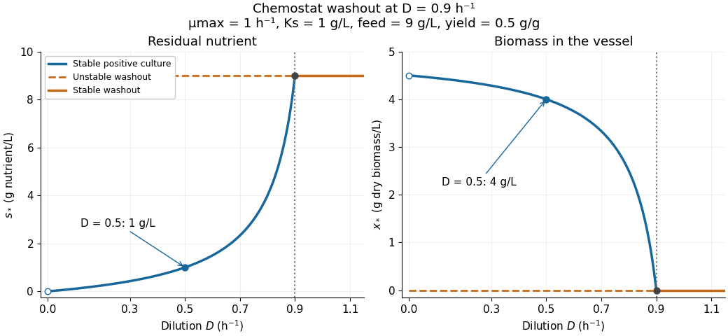
There is a useful exact simplification: the nutrient-equivalent concentration $z=s+x/Y$ satisfies $\dot{z}=D(s_{\mathrm{in}}-z)$, so $z(t)=s_{\mathrm{in}}+[z(0)-s_{\mathrm{in}}]e^{-Dt}$. This combines dissolved nutrient and the nutrient equivalent of biomass; it does not assert that these two variables account for every chemical constituent. In coordinates $(z,x)$, the Jacobian matrix at the positive chemostat steady state has eigenvalues $-D$ and $-{\mu }^{\prime }(s_{\ast })x_{\ast }/Y$, both negative. Hence the positive chemostat steady state is locally asymptotically stable. In the worked example the eigenvalues are $-0.5{\mathrm{h}}^{-1}$ and $-2{\mathrm{h}}^{-1}$.

The biomass yield $Y$ converts nutrient consumption into biomass production: consuming nutrient mass $m$ produces dry biomass mass $Ym$ under the assumed constant conversion. For $Y=0.5\mathrm{g}\text{ biomass}/(\mathrm{g}\text{ nutrient})$, consumption of $8\mathrm{g}$ of nutrient produces $4\mathrm{g}$ of dry biomass. Its numerical value depends on the measurement conventions; it is not a fraction of all feed mass converted into cells. With no separate maintenance consumption, biomass production $\mu (s)x$ requires nutrient consumption $\mu (s)x/Y$ in the chemostat balance.