
For a zero-mean stationary rough height, the mean first-order correction vanishes. At second order, the boundary derivative is . Averaging this expression using the power spectrum of surface height gives the displayed coherent reflection coefficient. Thus the root mean square height alone does not fix the coherent mean: the height correlation spectrum matters. For roughness varying slowly enough that in the integral, . A local random-height phase average needs this additional approximation and is not a general consequence of stationarity.
Positive feedback closes a causal loop whose net effect reinforces an initiating change. A loop with two inhibitory links can therefore have positive feedback. In signal transduction, a product that increases the activity of the enzyme making it illustrates reinforcement; the consequences depend on the full mathematical model, not just the loop sign. See signaling feedback.
A biological example is cell-cycle activation feedback. Cyclin B binds Cdc2, whose activity promotes activation of Cdc25; Cdc25 removes inhibitory phosphorylation from Cdc2, permitting further activation. Cdc2 also inhibits Wee1, an enzyme that inhibits Cdc2 through phosphorylation. That second return contains two inhibitions and therefore also has positive feedback. These are regulatory paths, not a claim that every connection is a single direct molecular encounter. [ref]
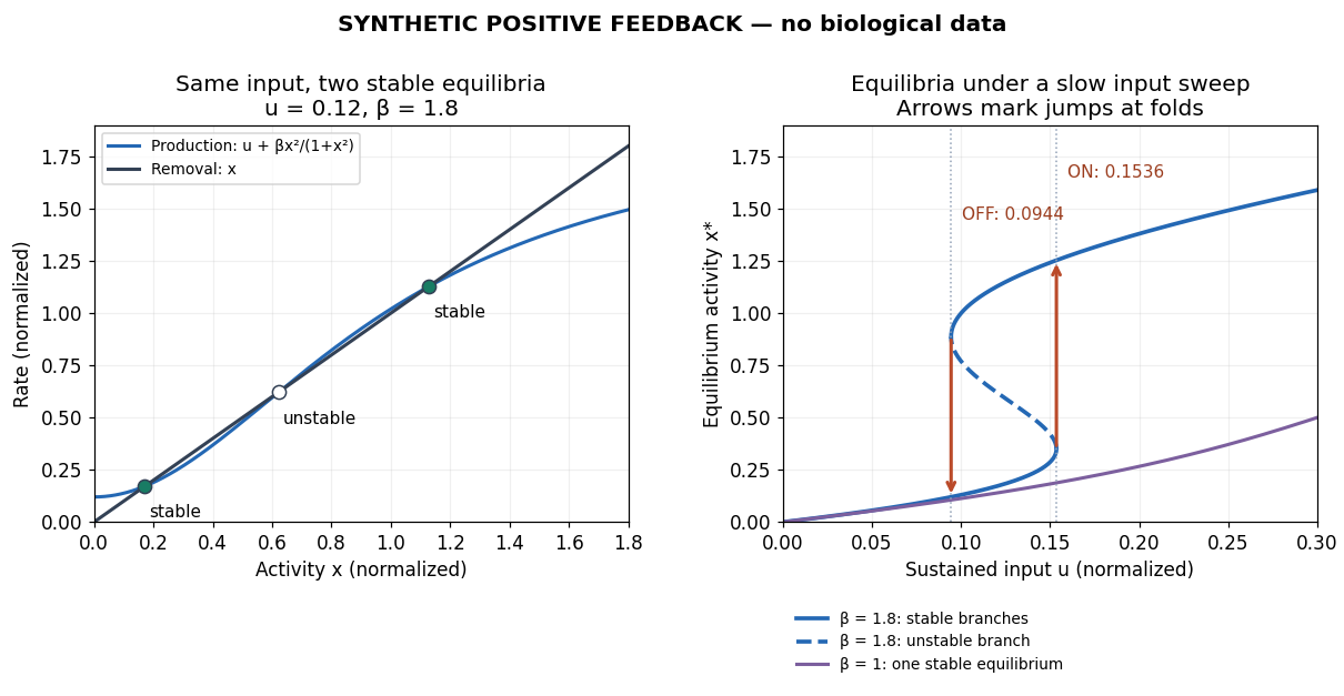
Reinforcement can preserve a decision after its initiating stimulus weakens: returning from the high state may require a lower input than entering it. The cell-cycle hysteresis experiment below tests this history dependence at matched cyclin B concentrations. A steep response alone is insufficient evidence of bistability, and finite observation times can make slow relaxation look like memory. A proposed switch must specify its input, readout and observation interval.

Negative feedback closes a causal loop whose net effect opposes an initiating change. In signal transduction, activation followed by a downstream inhibition of the earlier activating stage is one example of negative feedback. Loop sign alone does not establish asymptotic stability or complete signaling adaptation; see the worked signaling feedback example.
A useful biological example is chemotaxis feedback regulation: an Escherichia coli biological cell adjusts its response to a sustained attractant instead of remaining at its immediate response. Increased CheA activity promotes CheB phosphorylation; CheB reverses receptor methylation, opposing their activation. After attractant addition, reduced activity instead favors receptor methylation by CheR, restoring activity. This is a return from receptor activity to the machinery regulating that activity. The response need not return exactly at every dose. [ref]
A motivating measurement is the chemotaxis FRET assay. CheY and CheZ carrying yellow and cyan fluorescent tags were observed in immobilized Escherichia coli biological cells on a coverslip in a flow chamber. Adding and removing attractant changed the yellow-to-cyan emission ratio, reporting the association of phosphorylated CheY with CheZ. This measures a molecular readout upstream of motor behavior. Comparisons with biological cells lacking CheR, CheB, or both tested the dependence on receptor modification; these perturbations also change starting activity and sensitivity, so they are not pure changes of one feedback gain. [ref]
The later chemotaxis feedback regulation experiment used only the Tar receptor and nonmetabolizable methylaspartate, supplied and removed by flow. Long recordings separated slow recovery from incomplete signaling adaptation; correction for bleaching addressed drift in the optical readout. Activity recovered incompletely after sufficiently large additions, with detectable imprecision already at in that preparation. Restricting the receptor type and preventing consumption of the stimulus help interpret the perturbation, but limit transfer to other receptors and conditions. The readout infers CheA activity through CheY-CheZ association, rather than directly measuring every molecular step. [ref]
Negative feedback can also overshoot or sustain oscillations if its return arrives too late. The worked signaling feedback example gives the contrasting instantaneous case; the delayed negative feedback model below isolates the effect of timing. Loop sign describes causation, while asymptotic stability describes what happens to displacements over time.
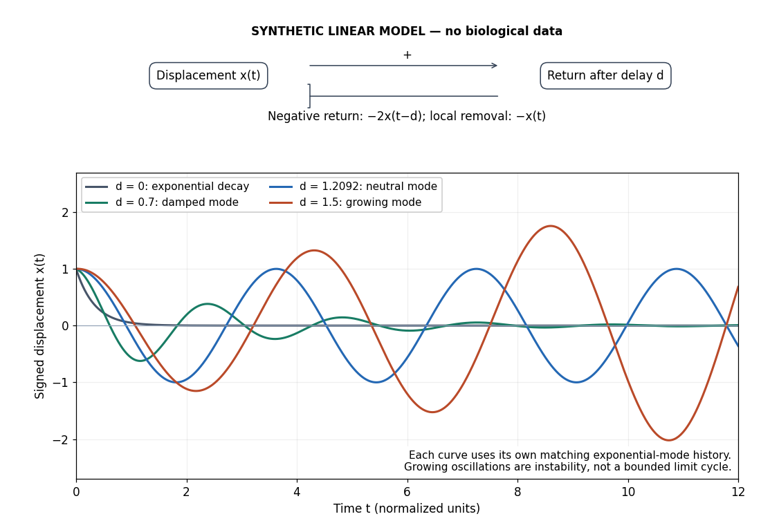
Negative feedback with an instantaneous or delayed return
. Original synthetic delay differential equation modes, not measured chemotaxis responses. All variables and time are normalized. The same negative return coefficient is used throughout; only its delay changes. Each curve has its own matching history. A growing oscillation signals instability of this linear mathematical model, not a bounded biological rhythm. Details.
Noise is unwanted variation in a signal. Whether a component is unwanted depends on the measurement task: suppressing fast variation helps only when that variation is expendable. White noise provides one mathematical model; it does not describe every source of disturbance. A linear filter may reduce some noise while also altering the desired signal.
A discrete-time signal assigns a value to each of a discrete collection of times, often indexed by the integers. Regular sampling at rate gives , so a sinusoid with normalized frequency cycles per sample has physical frequency . Discreteness of time does not itself require the amplitudes to be quantized; rounding the values is an additional operation. The Nyquist–Shannon sampling theorem gives conditions for recovering a band-limited continuous signal from its samples.
The computer bus paths specifying operations and coordinating progress, including requests and acknowledgments. Some control travels from initiator to target and some returns. In the diagram, bus arbitration requests and grants are shown separately from transfer control to distinguish choosing an initiator from executing its bus transaction.[ref]
Lecture 21: Buses and I and O. CS152 lecture 21, slides 22 and 33–36: control signals, sequencing, request and grant
The computer bus path carrying payload. A write sends data from the initiator to the target; a read returns data from the target. Owning the request path does not mean driving the data bus in both directions.[ref]
Lecture 21: Buses and I and O. CS152 lecture 21, slide 24: initiator commands, data in either direction
The computer bus path identifying the destination or location of a bus transaction. An initiator supplies an address; decoding selects the intended target. Address width describes the available address encodings, whereas data bus width describes how many bits can be carried at once.[ref]
In a channel whose transverse width does not depend on downstream position, the wetted area is and the integrated hydrostatic pressure force divided by density is . With cross-sectionally uniform velocity, volume conservation and momentum conservation give the displayed shallow water equations. Since , the two characteristic speeds are with . For , and the Riemann invariants are .
A hydraulic jump connects shallow supercritical flow to deeper subcritical flow while conserving discharge and momentum and dissipating mechanical energy. Its Rankine-Hugoniot condition uses the channel's actual area and integrated hydrostatic pressure, which depend on cross-sectional geometry.
For cross-sectional area and cross-sectionally uniform velocity, volume conservation gives , while hydrostatic inviscid momentum gives . Their characteristic speeds are . With , the robust compatibility equation is . Replacing by requires at fixed height; otherwise an explicit geometry term remains.
For a steady rectangular-channel flow with discharge , the shallow-water specific energy relative to the bed is . At fixed discharge and width, , where the Froude number satisfies . The minimum is , with . Without dissipation, is the conserved Bernoulli equation head for bed elevation .
In a sectionally uniform flow, a volume source per downstream length brings axial velocity . Momentum conservation gives the displayed source correction, with the wetted area. The head derivative is . Removing fluid at the local velocity preserves the head in this approximation. Adding fluid at rest does not: its acceleration reduces that head. The volume source alone cannot specify the momentum exchange without a velocity assumption.
For an outgoing simple wave into water initially at rest at depth , the incoming Riemann invariant is . Thus and the outgoing characteristic speed is . A boundary characteristic emitted at time is . Its envelope satisfies and . At a zero-velocity onset with positive acceleration, the leading-edge intersection is the displayed distance. Later characteristic curves can form a shock earlier elsewhere in a sufficiently strong waveform.
There are unlisted articles, also show them or only show them.