
Cited passages: David Tong, Statistical Physics, §§2.2.1 and 2.4: monatomic translational energy and diatomic rotation/vibration term counting.
Planck's law gives the spectral radiance of an ideal blackbody in thermal equilibrium at absolute temperature . It predicts how much power is carried in each small frequency or wavelength interval, per projected area and per solid angle. The whole curve is determined by : no material-specific parameter enters this ideal Planck function.
Writing for frequency in hertz and for wavelength in metres, the two forms of the Planck function areHere is the Planck constant, the Boltzmann constant, and the speed of light in vacuum. Their exact values in the International System of Units are , , and . [ref]
https://www.nist.gov/si-redefinition/meet-constants. NIST, Meet the Constants
The units matter: is measured in , whereas is measured in . Both are spectral radiance, rather than radiant exitance or energy density. To report per micrometre, multiply its per-metre value by ; a micrometre-wide interval is metres wide.
For a computed example, at and , the exponent is . Substitution into Planck's law gives , or per micrometre. At the same wavelength, the illustrative temperatures and give and in the latter units. These are ideal predictions for stipulated temperatures.
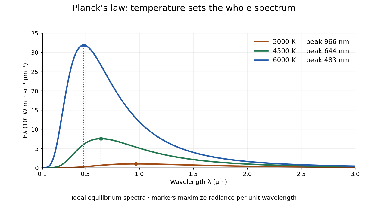

The key change of variables is . Corresponding positive intervals carry the same power, so andEqual-width wavelength intervals have unequal widths in frequency; the factor compensates for this. Merely replacing the horizontal-axis labels of by does not produce . This explains the frequency and wavelength peaks of Planck's law.
A short derivation uses the Boltzmann distribution for a single electromagnetic mode with thermal energies , . Put . The geometric series gives and mean thermal energy . The electromagnetic mode density in a box, including both independent polarization of an electromagnetic wave states of a photon, is per volume per unit frequency. Multiplication gives spectral energy density ; isotropy gives . This counts thermal excitation energy, excluding zero-point energy. [ref]
https://www.feynmanlectures.caltech.edu/I_41.html#Ch41-S3. Feynman Lectures, I.41.3, quantum oscillator and radiation
Planck's law connects quantum mechanics to a measurable radiation curve. Its small- limit is the Rayleigh-Jeans law, ; its large- limit is the Wien approximation, . The suppression at high frequency makes the total energy density finite. Integrating the curve gives the Stefan–Boltzmann law, while locating its peak gives Wien's displacement law. Thus one formula predicts both the spectral shape and the total emission.
An ice bath can absorb heat while its temperature barely changes: the heat converts ice into water. The latent heat of fusion quantifies this melting budget. For a pure substance at its equilibrium melting temperature and specified pressure , define it here per unit mass:Here and are the specific enthalpies of the coexisting bulk liquid and solid, and is enthalpy. For ordinary melting, , in ; an amount has a total fusion enthalpy in joules. A molar fusion enthalpy instead has units and equals , where is mass divided by amount of substance in . Always check the normalization before inserting a tabulated value into an energy balance.[ref] [ref]
For a closed system converting completely from solid to liquid at fixed pressure, with only pressure-volume work and negligible changes in bulk kinetic energy and potential energy, the first law of thermodynamics gives . Both endpoints are at : warming initially colder ice or subsequently warming the resulting water requires additional sensible heat. Since , the corresponding specific internal energy jump is , where ; includes the work associated with the change in volume. Heat is transferred energy, whereas enthalpy is a state function. [ref]
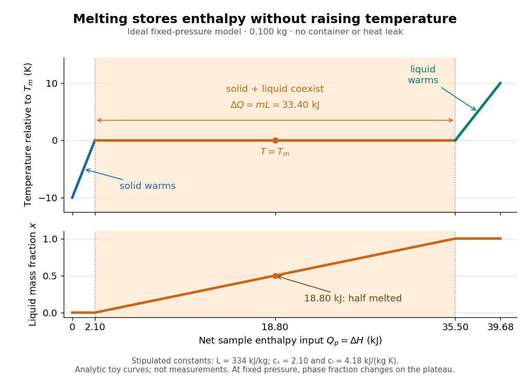

Let be the liquid phase fraction by mass, rather than by volume. Neglecting interfacial contributions to enthalpy, equilibrium phase coexistence at fixed pressure givesIn the model above, reaching takes of sensible heat; the plateau then absorbs , ending at a cumulative . At , half the mass is liquid and the temperature is still . The final warming takes another . The rounded and are inspired by the introductory ice-melting calorimetry values in Case Western's demonstration; constant properties and exact equilibrium throughout are stipulated model assumptions. [ref]
https://case.edu/artsci/phys/courses/demos/spec.htm. Case Western Reserve University, specific heat and heat of fusion demonstration
Within one thermodynamic phase, specific heat capacity at constant pressure is , in ; a sample's heat capacity at constant pressure is , in . The plateau is a finite enthalpy change at zero temperature change through varying , so neither a finite single-phase nor represents it. The heating curve needs separate sensible heat intervals and a fusion contribution. [ref]
The plateau assumes a pure substance, a stable bulk solid-liquid phase coexistence pair, fixed pressure, and sufficiently slow, uniform heating to remain near thermodynamic equilibrium. The total mass and composition must remain fixed, with negligible evaporation and no other phase transition. A fast heater can produce temperature gradients, so a local thermometer need not read the equilibrium . Neither nor is universal across pressures or compositions: common-pressure melting-point slope describes the pressure dependence of , while mixtures can melt over a temperature range as their coexisting compositions change. Their liquidus must be consulted instead of assuming a pure-substance plateau. [ref]
https://www2.tulane.edu/~sanelson/eens211/2compphasdiag.pdf#page=3. Stephen A. Nelson, Tulane, Two Component Phase Diagrams, pp. 2–4: melting ranges and liquidus
This makes ice useful as a temperature buffer: under these conditions it can absorb before the remaining solid mass disappears, after which the water warms. If a stipulated constant net input power goes entirely into melting, that buffer lasts . Reversing the equilibrium conversion releases the same fusion enthalpy during freezing. The beautiful thermodynamic connection is , with the specific entropy and absolute temperature: equal Gibbs free energies at phase coexistence allow different enthalpies and entropies. The nearly stationary thermometer hides a finite, measurable change of state. [ref]
The ergodic hypothesis identifies long-time averages of equilibrium observables along typical trajectories with averages over the invariant equilibrium ensemble at the same conserved quantities. In the microcanonical formulation, the ensemble is normalized phase-space measure on the energy surface. In a measure-preserving description, ergodicity means invariant measurable sets have measure zero or one; the Birkhoff ergodic theorem then equates time averages and ensemble expectations almost everywhere for integrable observables. This explains why statistical-mechanical ensembles can predict long-time measurements. A particular mechanical model still requires its own ergodicity assumptions; integrable idealized systems need not be ergodic.
Statistical mechanics connects microstates to macrostates through probability distributions. Its microcanonical ensemble, canonical ensemble and grand canonical ensemble specify different constraints on exchanges with the surroundings. An ensemble average describes repeated preparations under those constraints; it need not be the value in every individual preparation.
This makes the subject useful whenever tracking every microscopic detail would obscure the question being asked. To predict a heat capacity, we need how the expected value of energy changes with temperature, rather than a record of every unit's state. The partition function packages that calculation into one reusable object.
In his 1902 book, J. Willard Gibbs systematically developed the canonical ensemble. His preface contrasts following one system through time with studying a collection of systems with different microscopic conditions. Chapter IV defines the canonical ensemble through an exponential function of energy and establishes its normalization. This supplied a general strategy for predicting collective measurements by averaging over possible microscopic conditions, with the partition function organizing the calculation. [ref]
https://en.wikisource.org/wiki/Elementary_Principles_in_Statistical_Mechanics. Gibbs, Elementary Principles in Statistical Mechanics (1902), preface
[ref]https://en.wikisource.org/wiki/Elementary_Principles_in_Statistical_Mechanics/Chapter_IV. Gibbs (1902), Chapter IV, equations 90–93
A photon gas is a collection of photons described statistically as radiation. Here the equilibrium model is homogeneous, isotropic electromagnetic radiation in vacuum at temperature : each photon has energy , with momentum and frequency , and there are two independent transverse states of electromagnetic polarization. An absorbing cavity with walls at a common temperature provides a way to establish this thermal equilibrium. The bulk formulas assume cavity dimensions much larger than the typical wavelength , so the electromagnetic mode density in a box can replace individual cavity modes by a continuum. [ref]
https://davidtong.org/teaching/statistical-physics/statmechhtml/S3#S3.SS2. David Tong, Statistical Physics, §3.2: photon energies, polarizations and cavity equilibrium
The crucial constraint is whether photon emission and photon absorption, or other number-changing processes, can equilibrate the photon population. When they can, photon number is not an independently conserved quantity and the equilibrium photon chemical potential is . For each polarization and frequency, the mean occupation number then follows the Bose-Einstein distribution:If number-changing processes are ineffective but number-conserving interactions redistribute energy, a constrained Bose-Einstein distribution can instead have with chemical potential fixed by the number constraint. Thus thermal equilibrium with respect to energy exchange alone does not establish . The zero value can also persist in an already prepared Planck photon distribution during suitable subsequent evolution; continual photon emission is not required to preserve it. [ref]
https://academic.oup.com/ptep/article/2014/6/06B107/1560917. Hiroyuki Tashiro, CMB spectral distortions and energy release in the early universe (2014), §3.1: kinetic equilibration without full photon-number equilibration
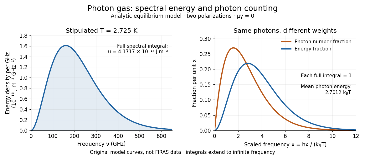
Combining with the two-polarization density of states, , gives the Planck photon distribution and the spectral photon energy density:Here is the spectral radiance in Planck's law; is stored energy density per unit frequency, not outgoing power per area. Their different units are connected by the full-sphere solid angle and the speed of light . The Boltzmann constant is , and is the Planck constant. [ref]
The equilibrium equation of state is particularly simple:The radiation constant is the same constant called in black-body radiation; is the Stefan-Boltzmann constant. An outline of the energy density calculation substitutes and uses . The radiation pressure follows because the angular average of the squared directional component of photon momentum is for isotropy; the thermodynamic derivation of blackbody radiation pressure supplies an independent route. These formulas describe the radiation contribution, not the cavity walls. The isotropic massless relation survives a different isotropic spectrum, whereas the coefficient in requires the zero-chemical potential Planck photon distribution.
For a computed example with stipulated , the photon energy density is and the radiation pressure is . The photon number density in the International System of Units isHere is the Riemann zeta function. The mean photon energy differs from the energy at the peak of a spectral curve: counting photons and weighting them by energy emphasize different frequencies. The calculations use the exact International System of Units values of the Planck constant, Boltzmann constant and speed of light. [ref]
https://www.nist.gov/si-redefinition/meet-constants. NIST, Meet the Constants: exact SI defining constants

A motivating observation is the cosmic microwave background spectrum measured by the Far Infrared Absolute Spectrophotometer (FIRAS) aboard COBE. Its apparatus used a polarizing Michelson interferometer, with one input viewing a roughly seven-degree sky patch and the other an internal blackbody. Scanning mirrors changed the optical path length difference; heat-sensitive detectors recorded the varying power, and Fourier transform spectroscopy recovered the spectral difference. Operation outside the terrestrial atmosphere removed atmospheric emission and absorption, while shielding and cooling the optics in a helium cryostat suppressed the instrument's own radiation. [ref]
https://lambda.gsfc.nasa.gov/data/cobe/firas/doc/FES4_APP_B.pdf. Mather, Fixsen and Shafer, Design for the COBE Far Infrared Absolute Spectrophotometer, apparatus and systematic-error controls
Absolute calibration came from moving an external blackbody into the sky aperture, filling the same beam used for the sky. This was an iron-loaded epoxy absorber shaped as a re-entrant cone. Repeated reflections made it a close approximation to a blackbody, while thermometers supplied its temperature. Mather and colleagues explicitly evaluated reflections, temperature gradients, radiation leaking through the material and leakage around its edge. These are limits on how faithfully the calibrator realizes thermal equilibrium radiation, rather than details that can be eliminated merely by calling it black. [ref]
https://arxiv.org/abs/astro-ph/9810373. Mather et al., Calibrator Design for COBE FIRAS (1999): absorber geometry and calibration error budget
During sky observations the internal blackbody temperature was adjusted to nearly null the spectral difference, reducing gain and drift errors. Fixsen and colleagues' 1996 analysis used calibrated spectra over wavenumbers to , about to . They separated the sky's spatially uniform component, its dipole and Galactic emission, and varied sky cuts and foreground templates as controls. The resulting cosmic microwave background spectrum agreed with a single Planck function, with reported RMS deviations below 50 parts per million of its peak brightness. This is a residual statistic over the analyzed spectrum, not a pointwise relative error bound at every frequency. [ref]
https://arxiv.org/abs/astro-ph/9605054. Fixsen et al., The Cosmic Microwave Background Spectrum from the Full COBE/FIRAS Data Set (1996), §§2, 5 and 5.3
The observation motivates using a photon gas as a physical model rather than merely a formal counting exercise. Its interpretation has a clear boundary: agreement with Planck's law constrains departures from an equilibrium spectral shape within the calibrated band and foreground assumptions; it does not directly measure radiation pressure or entropy density of a photon gas. Nor does it establish that today's cosmic microwave background is continually re-equilibrating with matter. A previously thermal spectrum can retain its Planck function shape as expansion of the universe lowers every photon frequency in the same proportion. The usefulness of the model is that one measured spectral temperature, together with its equilibrium assumptions, predicts energy density, radiation pressure, photon number density and entropy density of a photon gas consistently.
A thermal fluctuation is equilibrium variation of a random variable representing an observable. In a classical canonical ensemble with , assume and the state space measure are independent of , and fix temperature . Differentiating the normalized Boltzmann distribution givesThus the variance measures response to a conjugate field. For a two-state observable with energies , and , verifying the identity directly.
The same simple formula holds in a finite quantum system when the commutator of and vanishes. For noncommuting quantum observables, differentiation of the operator exponential produces an imaginary-time-ordered correlation function response rather than automatically . In a classical field theory, the spatial two-point analogue uses the connected correlation function.
Mean-field theory replaces fluctuating interactions with a self-consistent average field. For example, an Ising spin feels a field determined by the average neighboring spin magnetization; a self-consistency equation approximates the interacting Ising model. Neglecting correlated fluctuations can fail near a continuous phase transition. The mean-field approximation in Landau theory is a particular use of this general framework.
Cited passages: David Tong, Statistical Field Theory, §1.2.1, Spontaneous Symmetry Breaking: displayed nested limit and the immediately following explanation; David Tong, Statistical Field Theory, §1.2.1, discussion following equation (1.14): finite sums, analyticity, and macroscopic sharpness.
A call stack stores active procedure calls and the information needed to resume each caller, such as its return location and local variables. A call adds a frame; returning removes that frame and resumes the previous call. When depth-first search uses recursion, a frame also records where its adjacency list scan paused. The active frames describe a graph path from the starting vertex to the current vertex; finished calls have left the call stack, although their vertices remain marked as discovered.
DPPH is a neutral organic radical used as a spin reference in electron paramagnetic resonance (EPR), also called electron spin resonance (ESR). Its unpaired electron remains bound within the chemical species: “free radical” does not mean a freely moving electron. The DPPH electron spin resonance experiment makes its magnetic moment observable.
For the normalized sRGB calculations here, relative luminance is the linear-light weighted sumwhere are decoded linear-light components, not encoded code values. This is the sRGB calculation specified in W3C's WCAG 2.2 definition of relative luminance. It places reference black at 0 and reference white at 1; it does not by itself specify an absolute display light level.[ref]
https://www.w3.org/TR/WCAG22/#dfn-relative-luminance. W3C, WCAG 2.2, definition of relative luminance: sRGB decoding and weights
For a neutral sRGB shade, , and the weights sum to 1, so . For a coloured pixel, relative luminance can be encoded as a neutral sRGB shade with all three encoded components . This preserves the specified while discarding colour differences; it is one precisely defined grayscale conversion, not a unique way to turn all colour images into grayscale.
A numerical value retained for reuse by memoization. It is usable only while the spreadsheet formula and all its relevant inputs remain valid. After changing
A1 from 3 to 5, following outgoing directed edges finds exactly B1,B2,C1,D1. Invalidate their cached cell values before evaluating another requested result; install the new input value for A1. The cached cell values of A2 and E1 remain valid because neither has a directed path from A1.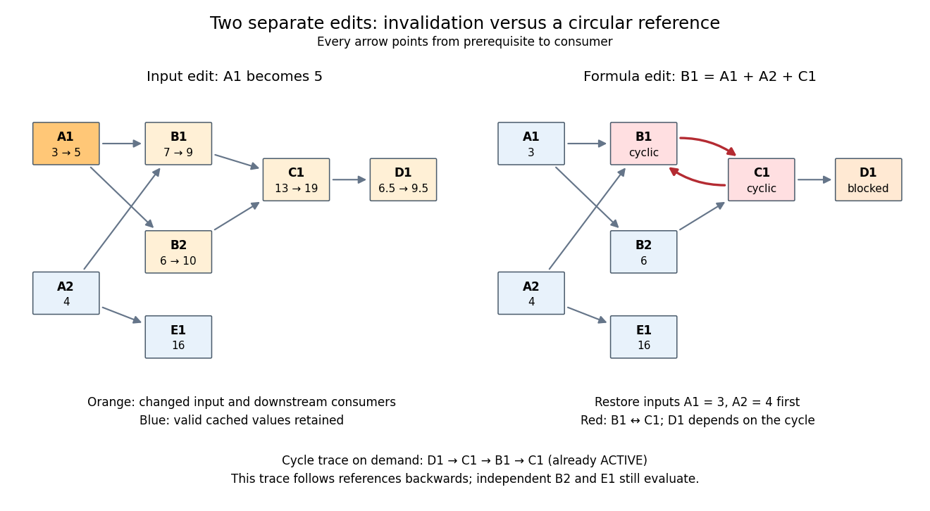
Downstream invalidation after an input edit, and a different formula edit creating a spreadsheet circular reference
. Details. 
One recomputation in the restricted topological order
B1,B2,C1,D1 gives . Four spreadsheet formulas are recomputed, while E1 stays at 16. Removing invalid values from the cache prevents a subtle error: a finished marker from the previous evaluation does not prove that the old value is correct after an edit. The affected set is conservative; a changed prerequisite might leave a consumer's value numerically equal, but this simple scheme still invalidates it. For a formula edit, update the incoming directed edges and corresponding outgoing consumer lists as well as invalidating the edited spreadsheet cell and its downstream consumers. Microsoft's documentation explicitly describes both direct and indirect dependents being marked for recalculation.[ref]Excel Recalculation by Microsoft. Dependence, Dirty Cells, and Recalculated Cells: paragraph beginning “When a structural change is made”; B1/A1 and C1/B1 dirty-cell example
For demand-driven evaluation, memoization combines with depth-first search. Each spreadsheet cell has one of three states:
UNSEEN means no valid cached cell value; ACTIVE means its evaluation is on the current call stack; FINISHED means a valid value is available. Initialize valid input spreadsheet cells as FINISHED. Start with all spreadsheet formulas UNSEEN, or retain only valid FINISHED entries after invalidation. The following original algorithm uses an ordered references list and an apply_formula operation for each spreadsheet formula:def value(cell):
if state[cell] == FINISHED:
return cache[cell]
if state[cell] == ACTIVE:
i = stack.index(cell)
raise CircularReference(stack[i:] + [cell])
state[cell] = ACTIVE
stack.append(cell)
try:
args = [value(p) for p in references[cell]]
cache[cell] = apply_formula(cell, args)
state[cell] = FINISHED
return cache[cell]
except Exception:
state[cell] = UNSEEN
raise
finally:
stack.pop()Requesting
D1 first makes D1,C1,B1 active, then reads the finished inputs A1,A2. B1 finishes at 7. Evaluating B2 reuses the finished value of A1 and finishes at 6; C1 finishes at 13 and D1 at . A later request for D1 immediately returns its cached cell value. The shared prerequisite A1 is not a directed cycle: it was finished before the second request. The crucial distinction is between a previously visited vertex and a still-active vertex. The exceptional path restores unfinished states while unwinding the call stack, so failed evaluations are not cached as successful results. MIT's depth-first search notes use stack-duration marks to distinguish an edge to an active ancestor and to detect a directed cycle.[ref]Lecture 14: Graphs II: Depth-First Search. Lecture 14: Graphs II: Depth-First Search, printed pp. 3–4: stack-duration marks and cycle detection
With adjacency lists and constant-time state/cache access, the structural work of a successful demand-driven evaluation is in big O notation, where and are the requested spreadsheet cells and their recursively reached prerequisites and references. Each reached spreadsheet formula is computed once; each reference is inspected once. This time complexity counts dependency bookkeeping separately from the cost of the arithmetic operations. Detecting a spreadsheet circular reference can additionally scan the current call stack once to report its witness.
The directed graph whose vertices are the spreadsheet cells and whose directed edges mean that the spreadsheet formula in references . Input spreadsheet cells have no prerequisites in this model. Retain both incoming references and outgoing consumers: depth-first search for evaluation follows incoming references backwards, whereas downstream invalidation follows outgoing consumers forwards. A directed path then expresses indirect dependence, and a directed cycle expresses a spreadsheet circular reference.
A mathematical expression stored in a spreadsheet cell, with references to other spreadsheet cells. In this example
=A1+A2 asks for addition, =2*A1 for multiplication, and =A2^2 for exponentiation. The evaluator in spreadsheet dependency evaluation assumes these spreadsheet formulas have already been represented by their ordered lists of referenced spreadsheet cells and operations on the resulting numbers; it does not execute arbitrary formula text.Copying a spreadsheet formula produces a new expression by adjusting its spreadsheet cell references. Copying only its displayed value produces a number instead. For example, copying the spreadsheet formula
=A2*B2 down one row gives =A3*B3; entering its former value in the next row would give neither the required relationship nor this example's correct subtotal .Einstein coefficients describe spontaneous emission, stimulated emission and absorption between atomic levels. With multiplying radiation energy density per frequency, thermal detailed balance gives and . Coefficients defined using mean specific intensity instead have a different normalization; specify the radiation convention.
The critical density of an atomic transition is the electron density at which its collisional de-excitation rate equals its spontaneous radiative decay rate. A multilevel atom requires summed competing rates rather than a single-transition ratio. This atomic density scale is distinct from cosmological critical density.
A radiative cascade is a sequence of downward photon-emitting transitions following excitation or recombination. Cascades feed lower excited levels and change their emitted line intensities. An effective recombination coefficient includes all relevant cascade paths under its stated optical-depth and density assumptions.
There are unlisted articles, also show them or only show them.