
A species can encompass many biological populations. A biological population specifies a set of organisms in a place and time; a biological strain identifies a maintained variant or lineage, often in a laboratory. A species name, a local census and a biological strain designation therefore describe different things. Multiple independently maintained cultures can also share the same biological strain designation.
For example, a culture identified as Escherichia coli K-12 MG1655 specifies more than the species alone. Two flasks inoculated from that culture are separate experimental biological populations; the separate containers do not establish two species or two different biological strains. This is an original experimental bookkeeping example, not a claim that every biological strain name encodes a complete genotype.
Species delimitation infers the boundaries and number of species from evidence. No single arbitrary percentage of nucleotide sequence difference is a universal boundary. Divergence within an old, widespread species can exceed divergence between recently separated species; geography and multiple kinds of evidence matter. [ref]
Species Concepts and Species Delimitation by Kevin de Queiroz. pp. 884–885, “Alternatives to the Traditional Properties”: divergence cutoffs and geographic differentiation
An original counterexample to a universal percentage rule: an assay could examine a strongly conserved gene in one comparison and a rapidly changing nucleotide sequence in another. Equal percentages then answer different historical questions. Even the denominator needs specifying: all sites, aligned sites, or only a filtered region? A threshold is an operational rule for a stated assay and group of organisms, whose errors need evaluating. It is not a definition that automatically transfers to every species.
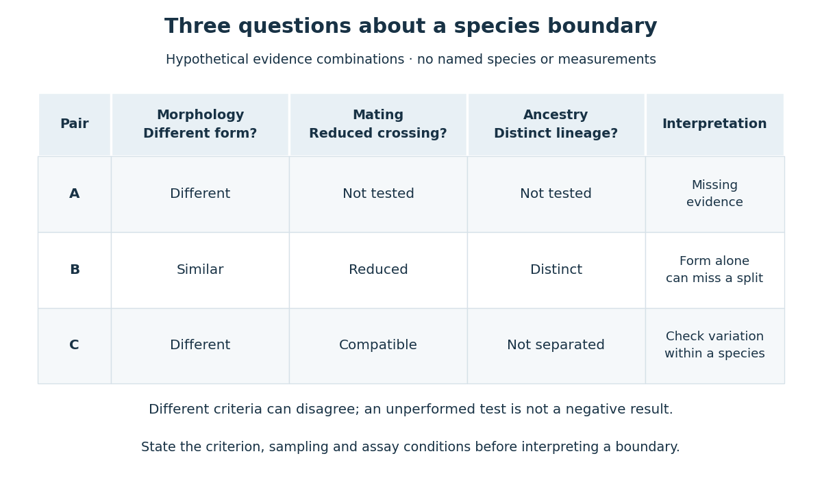
Contrasting operational evidence for species delimitation
. Original hypothetical comparison of morphology, mating and ancestry evidence. Each observation tests a different claim; the combinations are thought experiments, not a dataset or verdicts about named species. “Not tested” does not mean absent. Details.
The diagram's hypothetical pair B has similar morphology but reduced mating and distinct ancestry evidence. A morphological species concept could miss that distinction. Pair C instead has different morphology but compatible mating and ancestry that fails to separate the samples. That combination calls for checking variation in phenotype within a species. Pair A has only a structural difference observed: the other criteria remain untested. These examples show why missing evidence, disagreeing evidence and agreeing evidence require different interpretations.
A species concept states what should make organisms members of the same species; an operational criterion states what observations will test that claim. Reproductive isolation, distinguishable morphology and ancestry inferred through phylogenetics answer different questions. In a lineage-based interpretation, they are evidence for separation of evolving biological populations, and need not appear together. [ref]
Species Concepts and Species Delimitation by Kevin de Queiroz. pp. 880–883, Table 1, Figure 1 and “Conceptualization versus Delimitation”: distinguish defining properties from operational evidence
Reproductive isolation consists of barriers that reduce gene flow through sexual reproduction. Distinguish premating isolation from barriers after mating. Barriers before fertilization also include incompatible gametes; barriers after fertilization can reduce offspring survival or fertility. [ref]
Biology 2e by Mary Ann Clark and others. §18.2, “Reproductive Isolation”, opening paragraphs, gametic barriers and hybrid inviability/sterility
An assay should state which step it measures. Observing fewer cross-group matings does not measure offspring fertility; observing fertilization does not demonstrate that the offspring will reproduce. These distinctions make a partial barrier informative without declaring completed speciation.
A massive particle is nonrelativistic when its speed is small compared with the speed of light. Its energy expansion is . The leading momentum-dependent term is the classical kinetic energy.
A relativistic massive particle is described by a timelike worldline with proper-time four-velocity . In signature its normalization is and its momentum is . The relativistic charged-particle action adds electromagnetic coupling, whose variation gives the Lorentz force.
The laws of physics have the same form in all inertial frames; uniform absolute motion cannot be identified by experiments confined to an inertial laboratory. The invariant vacuum speed of light is a separate postulate. Together they motivate the Lorentz transformations of special relativity.
Merge sort is a divide-and-conquer algorithm that sorts a finite array by splitting it into contiguous halves, sorting each half using recursion, and combining the two sorted arrays with the merge algorithm. An empty or one-entry array is returned immediately. For length , put the first entries on the left and the remaining on the right; the brackets are the floor function and ceiling function. Always choose the left head on equal keys to obtain stable sorting. This is the split, sort, combine structure taught in the MIT lecture notes.[ref]
Lecture 3: Insertion sort, merge sort. 6.006 Introduction to Algorithms, Fall 2011 by Massachusetts Institute of Technology, 6.006 course staff; MIT 6.006 (2011), lecture 3: merge sort
Take the concrete input arrayThe tags identify the entries originally at indices and , counting from zero. Both keys are ; the tags are never compared. Reading downward in the figure follows the splits, then the returned sorted arrays. Arrows show dependencies; the level layout groups independent calls rather than giving their chronological execution order.
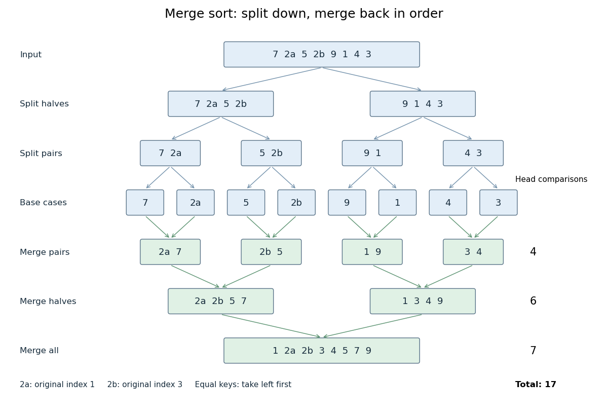

The first two halves are and . Their pairs split into one-entry base cases. Applying the merge algorithm gives the following fully worked return levels; each number in the last column counts only comparisons between two available heads.
| Returning level | Resulting sorted arrays | Head comparisons |
|---|---|---|
| Pairs | , , , | |
| Halves | , | |
| Whole array |
In the left-half merge algorithm, the head pairs are , and ; it takes , then appends . In the final merge algorithm, the head pairs are , , , , , and . It takes , then appends . Thus this precise version makes head comparisons and, ignoring identity tags, returns .
The elegance of merge sort is that it creates exactly the structure its next step needs: two smaller sorted arrays make the larger ordering inexpensive. Once the whole array is sorted, equal keys are adjacent and binary search can serve repeated queries. Stable sorting also retains information that the keys alone do not express. If the left-half merge algorithm instead takes the right head on the tie, it returns ; the keys are sorted but stable sorting has failed.
For time complexity, assume each key comparison, entry access and entry copy has constant cost. The merge algorithm processes entries in time. In Big O notation, the resulting recurrence relation isFor , the balanced levels contain entries each and there are returning levels. Each costs , so the worst-case time complexity is . For arbitrary , there are at most returning levels, each processing at most entries, giving the same bound. The worst-case number of head comparisons is also . Here is the base-two logarithm. The MIT notes give this level-by-level analysis for merge sort.[ref]
https://ocw.mit.edu/courses/6-006-introduction-to-algorithms-spring-2020/6d1ae5278d02bbecb5c4428928b24194_MIT6_006S20_lec3.pdf. MIT 6.006 (2020), lecture 3, page 5: merge sort analysis
The conventional array implementation uses a reusable buffer of entries for the merge algorithm, together with pending calls for recursion. Its auxiliary space complexity is therefore , beyond the original array. This bound describes that implementation. A linked list permits a merge algorithm that reconnects existing nodes; its storage accounting differs from copying array entries into a buffer.
For a short algorithm correctness outline, the empty and one-entry base cases are sorted. Assuming recursion correctly sorts both shorter halves, the merge algorithm returns all their entries in order. Equal keys within a half keep their relative order by the same argument applied to the smaller call; across halves, every left entry originally preceded every right entry, so taking left first preserves stable sorting. Both half-lengths decrease for , establishing termination.
Stable sorting preserves the original relative order of entries with equal keys. The entries may carry different names or other information even when their keys coincide. For example, sorting records by the numerical key gives : Ada remains before Cy. This is useful when a previous ordering contains information worth retaining, such as arrival order among equally ranked requests.
Radix sort sorts encoded sort keys a digit at a time. Its least-significant-digit version uses stable sorting on each successive digit, often by counting sort. For digits with possible values each, it takes time complexity in Big O notation, assuming constant-cost digit extraction and indexing. Stable sorting retains the ordering established by earlier digits when a later digit ties. Both digit access and the direct indexing in counting sort lie outside the comparison sort model, so these bounds do not contradict the comparison sorting lower bound.[ref]
Counting sort uses integer sort keys in directly as indices into an array of counts. Constant-cost counting and indexing give time complexity in Big O notation. To retain complete sorting records, cumulative counts locate their output ranges; filling each range from its end while scanning the input backwards gives stable sorting. Emitting bare sort keys from counts would discard associated data. The term matters when the key range is large.[ref]
11.2 Counting Sort and Radix Sort. Open Data Structures: An Introduction by Pat Morin; Theorem 11.7 and stability
For an original worked example, take complete sorting records and possible integer sort keys:The letters label the associated data, and are never compared. Both input and output array indices start at zero, so their valid positions are ; the count array has array indices . Stable sorting must produceThe equal-sort key groups retain and in arrival order. Counting sort prefix ranges explain where those groups belong; stable record placement in counting sort explains how to fill them without losing that order or the complete sorting records.
A comparison sort learns the ordering of sort keys only by comparing pairs. The keys are otherwise opaque: their numeric values, digits or encodings cannot choose an array index or a branch. It may move complete sorting records and retain previous answers. Merge sort and the adjacent-swap insertion sort are comparison sorts; counting sort and radix sort exploit additional information.
Insertion sort grows a sorted prefix of an array one entry at a time. In the adjacent-swap version, start with position , compare its current sort key with the preceding sort key, and swap the complete sorting records only when the right sort key is strictly smaller. Continue leftward until no swap is needed or the entry reaches position zero; then process original position . A tie stops the pass. This is the strict comparison and exchange rule in the authored implementation.[ref]
Take , where the subscript labels a complete sorting record and comparisons inspect only its sort key. Starting from index zero, the complete key-comparison trace is:
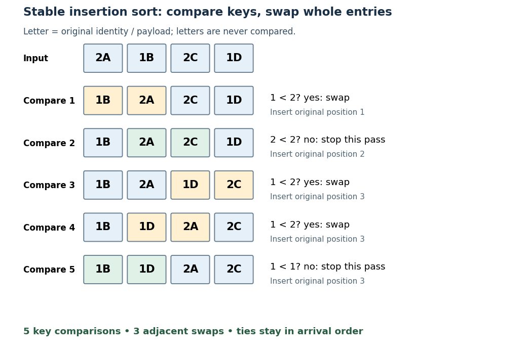

The loop invariant is that, before pass , positions satisfy sortedness and contain precisely the entries originally in that prefix. Moving the next entry left through strictly larger sort keys extends that prefix, and every swap retains sorting permutation preservation. Equal-key entries never cross, giving stable sorting. Each leftward step decreases the position, and each completed pass increases the prefix length, so the algorithm terminates.
With constant-cost key comparisons and swaps, reverse-ordered distinct sort keys cause comparisons and swaps. Thus worst-case time complexity is in Big O notation. An already sorted array needs only key comparisons for and no swaps. The adjacent-swap version uses constant auxiliary space complexity. Small or nearly sorted arrays can therefore make insertion sort useful despite its quadratic worst case.
The output of a sorting algorithm must be a permutation of the complete input sequence. For equal lengths , require a permutation of such thatEquivalently, the input and output have the same multiset of complete entries: each entry has the same multiplicity. Equality of the underlying sets is insufficient; and have the same set of values and the same length but different multisets. When tracking occurrences rather than contents, retain original identity labels to check that each one is moved exactly once. A swap preserves this multiset automatically; an overwrite need not.
For an output sequence of length , sortedness meansunder the chosen total order on sort keys. Its transitivity also gives whenever . An empty sequence and a one-entry sequence satisfy sortedness without any adjacent comparison. For longer sequences, checking adjacent pairs suffices; checking only the first and last sort keys does not. For example, passes an endpoint comparison but fails sortedness at . Sortedness alone says nothing about which input entries survived.
A sort key is the value extracted from a complete entry to determine its ordering. Model extraction as a function into a total order; compare and , while moving the complete entries. Ordering sorting records by an age field does not also compare their names. Repeated sort keys are allowed, so this induces equal-key groups even when the complete sorting records differ. Keep the sort key function and the comparison rule fixed throughout a sort; inconsistent comparisons need not admit any sorted result.
Dilution lowers a solute's concentration by adding solvent. For conserved amount of substance, molar concentration satisfiesBoth and are chemical solution volumes; is the final total, not the added solvent.[ref]
The proof is simply the definition applied before and after. Its useful assumptions are full transfer of the selected portion, no loss or gain of the counted solute, and complete mixing. An ideal chemical solution approximation is not required for this inventory equation. If chemical equilibrium redistributes dissolved chemical species, use a conserved analytical concentration or chemical element inventory rather than assuming each individual species is conserved. This conservation statement does not by itself preserve the pH: a chemical equilibrium may change as the chemical solution is diluted.
A solvent is the component designated as the medium of a chemical solution, commonly the component present in greatest proportion. Water is a common solvent, not a necessary one. A mixture of mostly ethanol with a little water can designate ethanol as solvent and water as solute. Chemical solutions can also be gas or solid mixtures; molecular nitrogen is the principal medium of ordinary well-mixed air. When proportions are comparable, state the convention explicitly.[ref]
The solvent is part of the final sample. Choosing it influences solubility and solvation; measuring its added volume alone does not determine the final chemical solution volume. Solvent and solute masses add in a closed account, whereas the final volume should be measured rather than inferred by adding pre-mixing volumes.
A solute is a component of a chemical solution distinguished from its solvent, typically present in a smaller proportion. There can be several solutes. A concentration must name both what is counted and the denominator: molar concentration uses amount of substance per final chemical solution volume; a solute-to-solvent mass ratio has another denominator.[ref]
“Added sodium chloride” and “dissolved sodium cations” describe different levels of the same inventory. Dissociation of an ionic compound changes the grouping of the particles; it preserves their chemical elements. A dissolved ion remains an ion, and dissolved sucrose remains molecular unless a separate chemical reaction occurs. Thus the name of the weighed solute need not be the name of every dissolved chemical species.
The concentration-based ionic strength is , where is each dissolved ion's concentration and its signed electric charge number. It has the same units as ; some formulas instead use the dimensionless ratio . All dissolved ions contribute, including those that balance the electric charge of a buffer solution's conjugate base. Ionic strength helps describe the interactions represented by activity coefficients. See Hippler and Metcalfe, activity coefficients and dimensionless ionic strength.
There are unlisted articles, also show them or only show them.