Basics of Space Flight (2017 edition) by Dave Doody Chapter 13: Navigation by  Codex 0 Created 2026-10-13 Updated 2026-11-05
 Basic Analysis: Introduction to Real Analysis, Volume II by Jiří Lebl 8.5 Inverse and implicit function theorems by Codex 0 2026-10-13
Codex 0 2026-10-13Online text: www.jirka.org/ra/html/sec_svinvfuncthm.html
Cited passages: Basic Analysis, Volume II, §8.5.1, Theorem 8.5.6 and the preceding circle example: local existence, uniqueness and derivative of an implicit graph.
Basic Analysis: Introduction to Real Analysis, Volume I by Jiří Lebl 1.2 The set of real numbers by Codex 0 Created 2026-10-13 Updated 2026-10-18
Codex 0 Created 2026-10-13 Updated 2026-10-18 Basic Analysis: Introduction to Real Analysis, Volume I by Jiří Lebl 2.1 Sequences and limits by Codex 0 2026-10-13
Codex 0 2026-10-13 Basic Analysis: Introduction to Real Analysis, Volume I by Jiří Lebl 5.1 The Riemann integral by Codex 0 2026-10-13
Codex 0 2026-10-13A conjugate base is what remains after a chemical acid donates one proton. In the conjugate acid-base pair , is the conjugate acid of ; accepting a proton reverses the conversion. For example, acetic acid loses a proton to give its conjugate base . Partners differ by one proton and one unit of electric charge; they need not always be neutral and negative. Hydronium/water and water/hydroxide are also conjugate acid-base pairs.
At a prescribed pH, the ideal dilute acid dissociation constant determines the partition of a monoprotic acid inventory between its chemical species:These dimensionless fractions sum to one. They are the weak acid dissociation fraction and its complement when the only acid-bearing chemical species are and . Equal fractions occur at in this ideal approximation. For nonideal chemical solutions, equality of thermodynamic activities need not mean equality of concentrations.
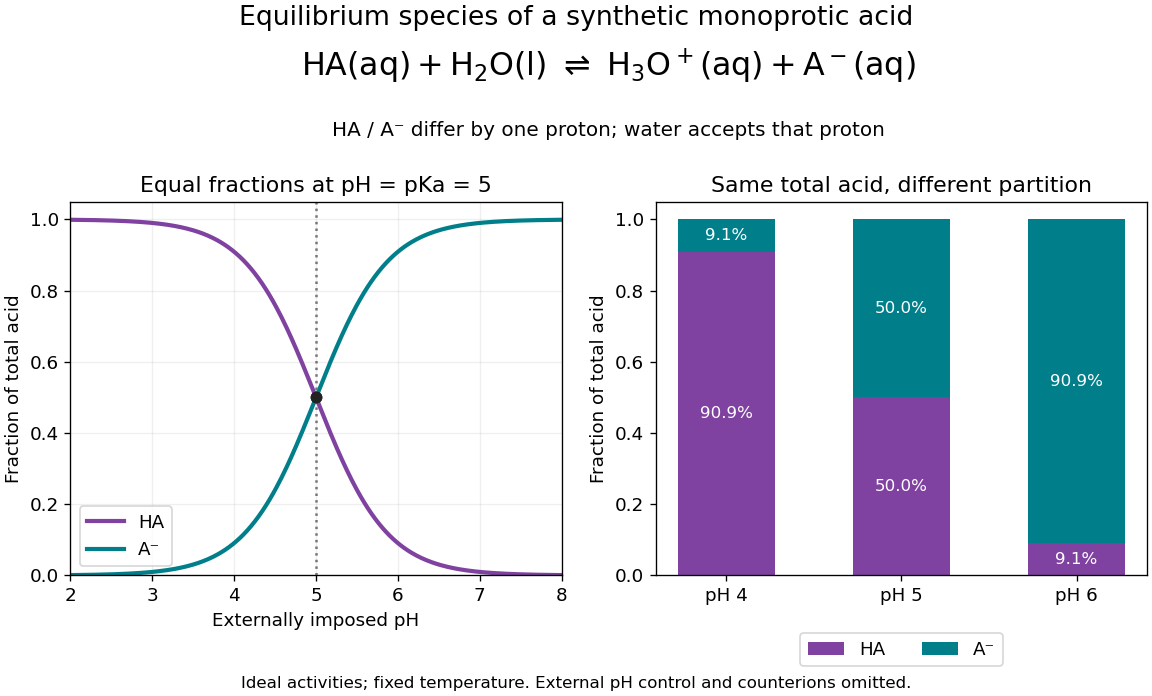
A synthetic monoprotic acid partitions between conjugate acid and conjugate base as imposed pH changes
. Details. For stipulated pKa , the conjugate base fractions at pH , and are , and . Here an external reservoir sets pH; its ions must supply the additional electric charge balance. The diagram omits those ions and water populations. It does not represent three pure samples at identical analytical concentration with freely chosen pH. In the latter experiment, the weak acid mass and charge balances determine pH as well as the partition.
Stellar parallax is the apparent change in a star's viewing direction caused by the observer's changing position. Nearby stars shift more against a distant reference background. In an ideal circular Earth orbit, the conventional annual stellar parallax uses a baseline of one astronomical unit, approximately the Earth-Sun distance. Two opposite observing positions, about six months apart, are separated by approximately two astronomical units. Their maximum angular separation is , so is half that excursion, not the full January-to-July shift. The observed excursion depends on the projected baseline and observing dates. [ref].
For the perpendicular baseline in the diagram, a right triangle giveswhere in the final expression is in radians. Combining the small-angle approximation with the parsec convention givesThus arcseconds implies parsecs, while the ideal six-month excursion is arcseconds. Geometry supplies this distance without assuming a luminosity or a particular stellar atmosphere.
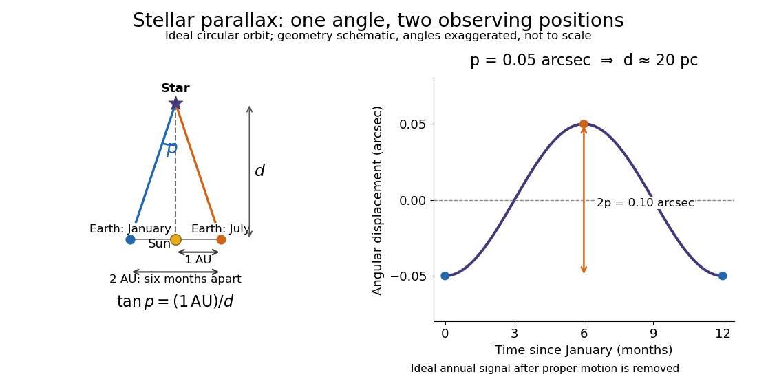


In practical astrometry, many observations separate the annual stellar parallax signal from proper motion, the star's own changing sky position. The Gaia DR3 catalogue reports stellar parallax and its uncertainty in milliarcseconds: arcseconds. A catalogue angle is a fitted measurement with measurement error. [ref].
For a positive stellar parallax with small standard deviation , first-order propagation gives . Thus with gives parsecs with parsecs, assuming systematic offsets are negligible. This linear estimate requires ; a reciprocal is nonlinear and does not generally preserve symmetric uncertainty intervals.
A point-like astronomical source has an angular extent negligible for the calculation or measurement being considered. The ideal mathematical limit concentrates its luminosity at one source-plane position. In gravitational lensing, this approximation permits divergent formal magnifications on a caustic; a finite source averages the magnification over its emitting area. An unresolved source need not have negligible size compared with the lens's caustic scale.
There are unlisted articles, also show them or only show them.