Every group representation of a finite group over a field whose characteristic does not divide the number of elements of the group is semisimple. Given an invariant subspace, averaging any projection onto it over the group produces an equivariant projection, whose kernel is an invariant complement.
A group representation is a group homomorphism from a group to the general linear group of a vector space. It realizes abstract group elements as invertible linear transformations.
The defining identities are and , so an inverse element is represented by a matrix inverse. A choice of basis gives a matrix representation, but the underlying action does not depend on that choice. The action need not distinguish every group element: the trivial representation sends all of them to .
A gauge field is a connection associated with a local symmetry in a gauge theory. Its gauge potential defines the internal-symmetry contribution to a covariant derivative. For an Abelian gauge field, the gauge field strength is .
A complex scalar field has distinct particle and antiparticle excitations and a global phase symmetry.
Perpendicular fields with and form a null electromagnetic field. The constant-field Lorentz-force generator is nilpotent, so its exponential terminates as a polynomial.
Both invariants of the electromagnetic field tensor vanish for this field class.
Relativistic hyperbolic motion in a uniform electric field by  Codex 0 Created 2026-09-24 Updated 2026-10-14
Codex 0 Created 2026-09-24 Updated 2026-10-14A particle released from rest in a constant electric field parallel to its motion follows a spacetime hyperbola and has rapidity proportional to proper time.
Lorentz boosts mix transverse electric and magnetic field components.
The four-potential combines the electric potential and magnetic vector potential as . The electromagnetic four-potential transforms underwhile the antisymmetric field tensor is unchanged.
Measure theory studies measures, which assign sizes to measurable sets, and the Lebesgue integral, which accumulates values weighted by those sizes. The same framework describes Lebesgue measure on the real numbers, counting measure on discrete collections, and probability measures on possible outcomes. The choice of measure determines what counts as large; the choice of sigma-algebra determines what can be measured.
A striking example separates size from proximity: the rational numbers in form a dense set with Lebesgue measure zero, although the whole interval has Lebesgue measure one. This distinction makes almost everywhere statements useful: exceptional null sets can be ignored in a Lebesgue integral even when they meet every open subinterval. The monotone convergence theorem and dominated convergence theorem then give precise conditions for passing a limit through an integral.
A historical starting point is Lebesgue's 1902 thesis, [ref]
https://www.ime.usp.br/~glaucio/mat5798/textos/aula1.pdf#page=2. Intégrale, Longueur, Aire (original title page reproduced in USP lecture notes)
. Its title connects integration with the geometric task of assigning sizes.A function on a convex set is a convex function if, for every and ,Geometrically, a line segment joining two points of its graph of a function lies on or above that graph of a function. The convex set condition ensures that the intermediate input stays in the domain of a function. An affine function satisfies the defining inequality with equality.
For the quadratic function , the inputs and have equally weighted arithmetic mean . Evaluating at the arithmetic mean gives , whereas averaging the outputs gives . Averaging first saves one unit in this example. More generally, direct expansion givesThis identity proves convexity and also shows exactly when its defining inequality is strict.
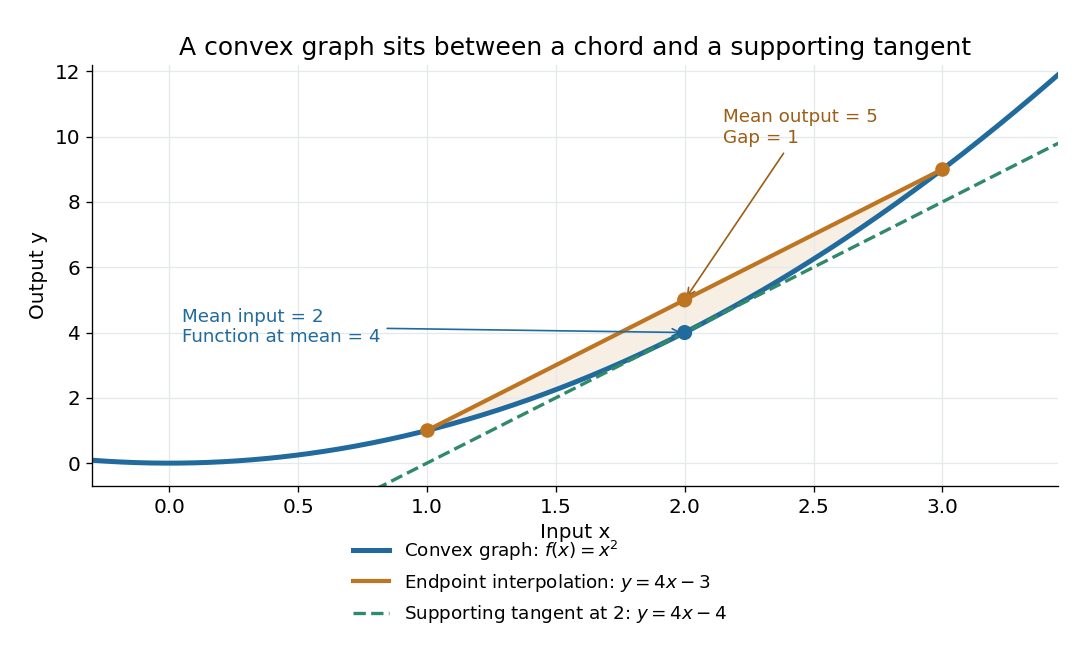
The graph of a convex quadratic lies below its endpoint interpolation and above its supporting tangent
. For , the line segment through and has height at , while the graph of a function has height . The tangent line is an affine minorant: everywhere. Details.
For a differentiable convex function, the tangent line in one dimension, or the corresponding supporting affine function in several dimensions, lies below the entire graph of a function. This is the subgradient inequality. The equivalent geometric statement is that the epigraph, consisting of points on or above the graph of a function, is a convex set. These characterizations are developed in Boyd and Vandenberghe's convex-function slides, sections 3.1–3.4.
Convexity does not require differentiability: the absolute value function is a convex function with a corner at . When a function is twice continuously differentiable on an open interval, it is a convex function exactly when its second derivative is nonnegative throughout that interval. In several dimensions, the corresponding criterion on an open convex set is that its Hessian matrix is positive semidefinite everywhere. The domain of a function matters: is a convex function on , but not on all of . A strictly positive second derivative is sufficient for strict convexity, but is not necessary: is a strictly convex function although its second derivative vanishes at .
The usefulness of convexity is that local information can certify a global conclusion. Every local minimum of a convex function on a convex set is a global minimum: if a lower value existed elsewhere, the defining inequality would produce lower values arbitrarily close to the proposed local minimum. For a differentiable convex function on an open convex set, a zero gradient therefore certifies a global minimum. Strict convexity gives uniqueness when a global minimum exists; it does not supply existence by itself. These facts explain the role of convex functions in convex optimization.
A convergent subsequence of is a sequence with strictly increasing indices that converges to a limit.
For a nonempty set , a real number is its infimum precisely when it is a lower bound and every other lower bound is at most . It is the greatest lower bound, not necessarily the minimum.
For , zero is a lower bound. Every positive candidate fails: the Archimedean property gives an integer , hence . Thus , although zero is never a member of . This is the lower-edge counterpart of approximating an unattained supremum.
For a nonempty set , a real number is its supremum precisely when it is an upper bound and no smaller real number is an upper bound. It is unique: two least upper bounds must each be no greater than the other.
For , every number at least one is an upper bound, and none smaller than one bounds the whole set. Thus , although . For , that same supremum is also the maximum. The approximation property of a supremum supplies witnesses arbitrarily close to an unattained upper edge.
There are unlisted articles, also show them or only show them.