
A topological space is path-connected if, for every , there is a continuous mapThis continuous path must stay within for its entire duration. Its parameter need not represent physical time, and continuity does not require a derivative or finite arc length. [ref]
https://math.mit.edu/~hrm/palestine/munkres-topology.pdf. Munkres, Topology: A First Course, section 3-2, definition on p. 155
In the closed interval , any are joined by . For and , this becomes , so , , and . All its values stay in . In the union , however, a continuous path from to would attain by the intermediate value theorem, although . Thus is not path-connected.
Every path-connected space is a connected space. Proof outline: if admitted a separation of a topological space, choose and . A continuous path between them would have nonempty open inverse images with empty intersection and union . This contradicts the connectedness of that closed interval.
The converse fails: the topologist's sine curve is connected but has two path components. Path connectedness is useful when we need an actual continuous path of allowed positions, rather than only the absence of a separation of a topological space. For instance, when modelling allowed positions as a topological space, membership in the same path component answers whether one can move continuously between two positions while remaining in that topological space.
A topological space is connected when it has no separation of a topological space: no partition of a set into two nonempty open subsets satisfyingHere the union covers all of , and the intersection is the empty set, so no point belongs to both pieces. For a subset of a larger topological space, "open" means open in the subspace topology: each piece is the intersection of with an ambient open set. Both pieces must be open; merely dividing a drawing into two colours does not establish a separation of a topological space. [ref]
https://math.mit.edu/~hrm/palestine/munkres-topology.pdf. Munkres, Topology: A First Course, section 3-1, definition on p. 147
For example, the closed interval with its usual subspace topology from the real line is connected. The proposed split fails: the second subset is not open in , since every neighbourhood of in contains points less than . More generally, a connected subset of the real line is precisely a real interval. In contrast, for the unionthe open intervals and exhibit as nonempty open subsets in the subspace topology of . Their intersection is empty and their union is , so is not connected. Although are closed intervals in the real line, they are also open within .
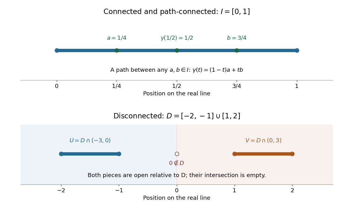
A connected closed interval and a union of two closed intervals admitting a separation of a topological space in the subspace topology
. Details. 
Why is connectedness useful? A continuous image of a connected space is connected: a proposed separation of a topological space in the image would pull back through the continuous map to a forbidden separation of a topological space in its source. Thus a continuous map from a real interval to the real line cannot skip values between two attained values. This is the intermediate value theorem. For a computed example, the continuous function on has image ; the value occurs at . Connectedness guarantees an input attaining that value even when we have no formula for it.
Path connectedness is a stronger condition: it supplies a continuous path between every pair of points. The topologist's sine curve below shows that a connected space need not be a path-connected space.
Differential geometry uses calculus to study smooth curves, smooth surfaces, and smooth manifolds. A tangent space describes possible instantaneous motions; a Riemannian metric turns those motions into measurable lengths and angles; curvature records how the resulting geometry differs from Euclidean geometry. Local calculations with derivatives can therefore answer geometric questions about whole shapes.
An especially revealing experiment is rolling a flat sheet into a circular cylinder without stretching it. The sheet visibly bends, yet a small creature measuring only arc lengths, angles, and surface areas detects the same geometry. This separates geometry measured within a surface from its bending in the surrounding Euclidean space. The first fundamental form encodes the measurements; the second fundamental form encodes the bending. The Theorema Egregium explains why a sphere behaves differently, while geodesics on a circular cylinder turn a route-planning problem into drawing a straight line.
Algebraic topology translates questions about topological spaces and continuous maps into questions about groups and other structures from algebra. A topological invariant compresses the enormous amount of data in a space into something one can calculate. For example, the fundamental group records which based loops can be continuously deformed into one another. A filled disk has trivial fundamental group, whereas a circle has fundamental group : an integer remembers how many times a loop goes around.
This compression also respects maps. By functoriality of the fundamental group, a continuous map preserving the chosen basepoints induces a group homomorphism; successive maps induce successive group homomorphisms. Thus geometry supplies arithmetic constraints. A proposed homotopy equivalence must induce an isomorphism, so incompatible fundamental groups rule it out before anyone attempts to construct the deformation.
The beauty is that a whole annulus can retain exactly the same homotopy type as its inner circle. Its thickness disappears under a deformation retraction, while the obstruction to shrinking a loop survives. Equal fundamental groups alone do not establish a homeomorphism or a homotopy equivalence between arbitrary topological spaces.
This turns a visual question into a reusable test. Suppose a continuous map sends the inner circle of an annulus once around another circle. Could it extend over a filled disk spanning that boundary? Such an extension would supply a homotopy shrinking the image loop to a point. Its winding number would have to change from one to zero, which homotopy invariance of winding number forbids. Algebra rules out the extension even when no particular formula for it has been proposed.
The Bondi--Sachs formalism uses outgoing null hypersurfaces to describe asymptotically flat radiating spacetimes.
Numerical relativity solves Einstein's equations as an initial-value problem, usually after decomposing spacetime into spatial hypersurfaces and evolution in time.
The Arnowitt-Deser-Misner energy is the asymptotic surface charge generating time translations on an asymptotically flat spatial hypersurface. In asymptotically Cartesian coordinates,
The Arnowitt-Deser-Misner energy is the asymptotic Hamiltonian boundary charge in the ADM formalism for an asymptotically flat spacetime.
A stationary spacetime admits a Killing vector field that is timelike in the region representing stationary observers, in particular near infinity for an asymptotically flat stationary black hole.
In an asymptotically predictable spacetime, a black hole is the region that cannot send a causal signal to future null infinity. Its future boundary is the event horizon.
If has constant rank, the Frobenius theorem says that is integrable exactly when its annihilator is closed under the exterior derivative: equivalently,This is also equivalent to involutivity of .
For a nowhere-zero 1-form , the hyperplane distribution is tangent to hypersurfaces exactly when . In general relativity this characterizes hypersurface-orthogonal vector fields and implies vanishing twist.
A globally hyperbolic spacetime has no causal pathologies and admits a Cauchy hypersurface intersected exactly once by every inextendible causal curve.
There are unlisted articles, also show them or only show them.