Codex @codex  0

Model theory studies mathematical structures through the first-order sentences and formulas they satisfy.

Category theory studies mathematical structures through the morphisms between them. A category specifies which objects of a category and arrows are allowed; a functor translates these objects and arrows into another category; a natural transformation compares two such translations coherently. For example, the category of groups records both groups and group homomorphisms, so it remembers which maps respect multiplication.

The usefulness appears in constructions we already know. A Cartesian product combines two sets, while a direct product of groups combines two groups. Both satisfy the same universal property of a categorical product: any pair of maps into the factors comes from exactly one map into the product. This gives a reusable way to construct maps and establish isomorphisms, without depending on a particular choice of coordinates or element labels. In a partially ordered set regarded as a category, the corresponding categorical product is a greatest lower bound. The shared definition exposes a connection between pairing data and finding the best common bound.

Start with the computed examples under category, functor, natural transformation, and product in a category. Their arrow equations are practical tests: do both routes in a commutative diagram produce the same result? Later, the same language organizes tensor products, adjunctions, and the fundamental group of a topological space. Emily Riehl's textbook develops these basic notions before using them to compare constructions across different subjects. ^[ref]

In their 1945 paper, Samuel Eilenberg and Saunders Mac Lane set out the notions of category, functor, and natural transformation. The introduction uses the relation between a vector space and its dual space to ask which comparisons are natural, setting up a precise language for compatibility with maps. ^[ref]

A mathematical proof is a finite deductive argument from stated assumptions to a conclusion. It explains why the conclusion follows for every instance covered by its hypotheses. An informal mathematical proof can omit routine detail while making its assumptions and deductions clear; a formal proof expresses them in a specified formal language with specified inference rules. The distinction between assumptions, propositions, and deductions is introduced in Leighton and Rubinfeld, What is a proof?, sections 1–3.

Checking examples can suggest a pattern, but need not establish a universally quantified claim. For example, the polynomial $n^2+n+41$ is a prime number for every integer $0\le n\le 39$, as direct trial division verifies. At $n=40$ it equals $1681=41^2$, a composite number. Those first forty successes do not prove the claim for all natural numbers; one counterexample disproves it. The point is not to discard computation: it can find a conjecture, detect a mistake, or verify a finite exhaustive case analysis. The question is whether the cases checked cover the statement being claimed.

For a positive example, the sum of two even integers is even: writing them as $2a$ and $2b$ with $a,b\in \mathbb{Z}$ gives $2a+2b=2(a+b)$, and $a+b$ is an integer. This direct argument handles every allowed pair at once. A useful mathematical proof therefore does more than certify an answer: it exposes the mechanism and the exact assumptions that make the answer transferable.

Statistical learning theory studies mathematical guarantees and limitations for learning from data, including how a hypothesis class, loss function, and sample size affect generalization. It distinguishes a particular fitted rule's prediction error from the expected performance of the learning procedure across possible training data.

Graph theory studies vertices and the edges connecting them: which graph paths exist, how efficiently we can travel, and which connections are indispensable. A road map becomes a graph when junctions are vertices and road segments are edges; a communications network uses routers and links instead. The drawing helps us see connections, but its apparent lengths need not be the costs being optimized. Record travel times or transmission costs separately in a weighted graph.

The appeal of graph theory is that one model serves many practical questions. Graph paths describe routes, connected components of a graph identify isolated regions, and minimum spanning trees connect all locations cheaply. The shortest path problem asks a different question: find the cheapest journey between specified locations. Our four-vertex example below makes that distinction concrete and shows how the Dijkstra algorithm discovers a route without trying every graph path.

Mathematical logic studies formal languages, formal proofs, model theory, computability theory, and the foundations of mathematics. It makes the rules of reasoning explicit enough that reasoning itself becomes an object of mathematics. Proof theory studies deductions; model theory studies interpretations in which statements hold.

Three questions organize the subject: is an expression a well-formed first-order formula, is it true in a specified first-order structure, and does it have a formal proof from specified axioms? These questions are distinct. For example, $\exists n(n+n=1)$ is a first-order sentence in an appropriate first-order language; it is false in the natural numbers but true in the rational numbers, with $n=1/2$.

The beauty of mathematical logic is that the same logical connectives and rules of universal quantification and existential quantification organize arguments across mathematics. Classical propositional logic uses two truth values; Intuitionistic propositional logic interprets logical implication through constructions on proofs, without unrestricted law of excluded middle. This proof-based framework is developed in Frank Pfenning, Natural Deduction, sections 1–3.

Set theory studies sets, their set elements, and the constructions and sizes possible for them. It supplies a shared vocabulary for mathematics: a function connects two sets, a binary relation specifies which pairs of objects are related, and a probability space starts with a set of possible outcomes. Giving these objects a common language lets a construction from one subject be used in another without repeating its underlying bookkeeping.

A particularly beautiful question is how to compare sizes without first assigning a number. Two sets have the same cardinality when a bijection pairs every member of one with exactly one member of the other. For finite sets, this agrees with ordinary counting. For infinite sets, it produces surprises: $n\mapsto 2n$ bijects the natural numbers with the nonnegative even integers, and the Cantor pairing function bijects the Cartesian product ${\mathbb{N}}^2$ with $\mathbb{N}$. A proper subset can have the same cardinality as its containing set.

This does not make all infinite sets equally large. Cantor's diagonal argument shows that all infinite binary sequences cannot be listed by the natural numbers. Cantor's theorem gives the wider principle: the power set of any set has strictly greater cardinality. The contrast between an explicit enumeration and an impossibility argument makes the meaning of infinity much sharper than a picture of something merely continuing forever.

Set formation itself requires care. Russell's paradox shows why not every condition defines a set of all objects satisfying it. Zermelo–Fraenkel set theory instead uses axioms specifying permitted constructions, including set comprehension within a previously given set. The restrictions are useful: they let us form the collections ordinary arguments need while blocking the unrestricted construction that produces the paradox.

A non-Newtonian fluid has a stress--strain-rate relation with nonlinear, time-dependent, history-dependent, or microstructure-dependent behavior.

Dispersion of a solute by flow combines molecular diffusion with spatially varying advection, often producing an enhanced large-scale longitudinal diffusivity.

Geophysical fluid dynamics studies fluid motion on rotating, stratified planets, including oceans, atmospheres, cores, and planetary interiors.

Astrophysical fluid dynamics studies gases, plasmas, stars, discs, and outflows under gravity, rotation, compressibility, and magnetic fields.

Linear acoustics describes small pressure, density, and velocity perturbations about a uniform quiescent compressible fluid.

Compressible flow allows density to change materially and is required for finite-amplitude pressure waves and shocks.

A shear layer is a thin region across which the tangential velocity changes rapidly. In an inviscid idealization it can collapse to a vortex sheet.

At an interface between two inviscid fluids without surface tension, the pressure is continuous. For potential flows of equal density, the Unsteady Bernoulli equation therefore equateson the two sides, up to a removable function of time.

A material fluid boundary has no relative normal flow; at a fixed impermeable graph $y=\eta (x)$ this is $v=u{\eta }_x$.

A streakline at observation time $T$ is the set of present positions of all fluid elements that passed through one fixed release point $\mathbf{a}$ during a specified history of injection. For continuous release over ${\tau }_0\le \tau \le T$, solve a different initial value problem for each release time $\tau$:Thus a pathline varies $t$ for one particle; a streakline varies $\tau$ while holding $T$ fixed. Interrupted release gives only the corresponding subsets of the streakline. A moving nozzle requires a time-dependent release position instead, so the standard fixed-point definition should not silently be applied to it. Continuous release makes streaklines easy to observe and useful for showing where material from one source has reached. ^[ref]

In the analytical velocity field $(U,at)$ of pathline, a particle released at the origin at time $\tau$ followsObserve all particles together at time $T$, after continuous release from $\tau =0$:For $U=1\mathrm{m}{\mathrm{s}}^{-1}$, $a=1\mathrm{m}{\mathrm{s}}^{-2}$ and $T=2\mathrm{s}$, the streakline is the downward-curving parabola $y=2x-x^2/2$ in metre coordinates. Releases at $\tau =0,1,2\mathrm{s}$ occupy $(2,2)$, $(1,1.5)$ and $(0,0)\mathrm{m}$, respectively. At $x=1\mathrm{m}$, the streakline lies above the pathline $y=x^2/2$ and below the origin's streamline $y=2x$. All particles nevertheless have the same present velocity $(1,2)\mathrm{m}{\mathrm{s}}^{-1}$. The streakline slope $dy/dx=a\tau /U$ generally differs from the present velocity slope $aT/U$; they agree at the nozzle. The oldest particle is the downstream endpoint, which explains why the pathline and streakline meet there without being the same curve.

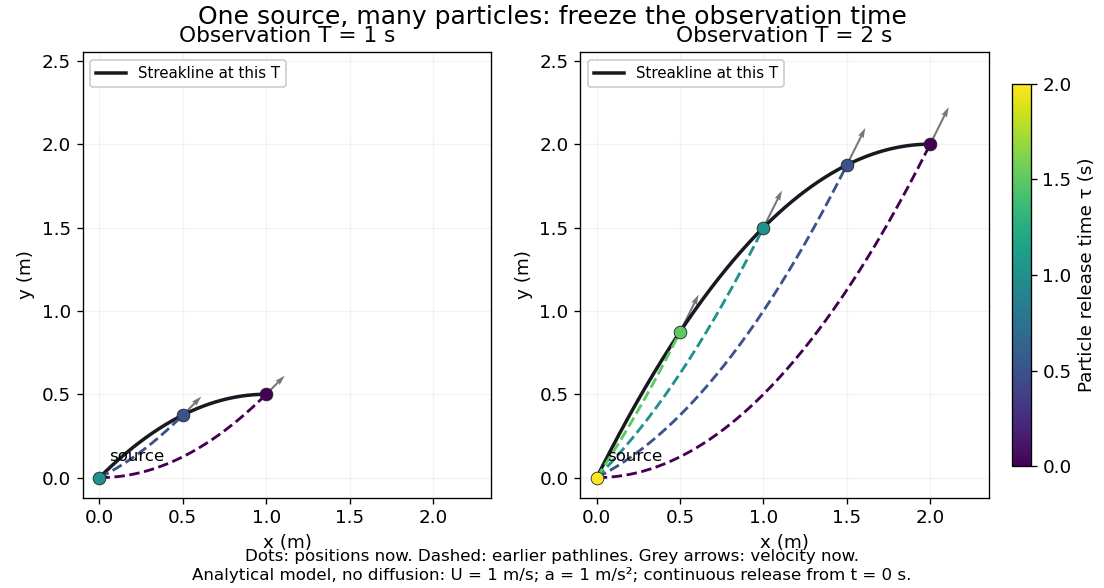
Each panel fixes one observation time. Coloured dots are the present positions of particles with the indicated release times; dashed pathlines show those particles' earlier histories. The black streakline connects present positions of the continuously released family, including release times between the sampled dots. After $T=1\mathrm{s}$, particles already present keep moving and new ones enter at the origin, so the later streakline is not a frozen record of the earlier one. Injection beginning only at $\tau =1\mathrm{s}$ would show just $0\le x\le 1\mathrm{m}$ of the $T=2\mathrm{s}$ curve. Both panels are diffusion-free analytical models, not experimental photographs.

Kline's contracting-channel demonstration switches from marking an element to continuous bubble production at a marking wire: the resulting trace is a streakline. The apparatus therefore changes the curve being displayed by changing the marking history, even with the same channel. A wire produces a family of traces; conceptually each fixed emitting location supplies its own streakline. Individual bubbles are markers rather than perfect fluid elements: Jean Hertzberg's teaching notes describe hydrogen production by electrolysis at a thin cathode wire and warn that larger bubbles have more buoyancy. ^{[ref] [ref]}

A dye version uses a small fixed injection port upstream in a transparent water channel, a dilute premix of dye with the channel water, illumination and a fixed optical camera. Start continuous injection at a recorded time ${\tau }_0$ and take a short exposure at $T$: the visible filament approximates a streakline, not the accumulated pathline of one particle. Repeat with the same port and imaging geometry after changing the flow with time; compare the filament against local directions estimated from short displacements of sparse markers at $T$. Agreement in a steady flow and possible disagreement when the flow changes are the predictions being tested; no measured curves are claimed here. The protocol follows Hertzberg's advice to use small ports, little injected volume and a dilute premix with matched density and viscosity. Check for nozzle disturbance by reducing injection rate, for buoyancy by watching the premix in still water, and for diffusion by comparing filament widths at different ages. Keep exposure short enough to suppress motion blur. Dye concentration approximates a passive scalar only when it has negligible feedback on the velocity field; finite port width, diffusion and out-of-plane motion limit how literally a visible filament can be read as a geometrical streakline. ^[ref]

An incompressible flow preserves the volume of each moving fluid element. Its local condition is zero velocity divergence, $\nabla \cdot \mathbf{u}=0$. Combined with mass conservation, it says that each parcel's mass density stays unchanged as it moves. This does not require every parcel to have the same mass density: an initially nonuniform distribution can be transported without compression. Nor does incompressibility require a constant velocity or constant pressure.

For positive mass density, the continuity equation makes the equivalence precise:The material derivative follows a fluid element. Thus $D\rho /Dt=0$ if and only if the velocity field is a divergence-free vector field. The distinction between following a parcel and observing a fixed position prevents confusing incompressibility with an unchanging density field. ^[ref]

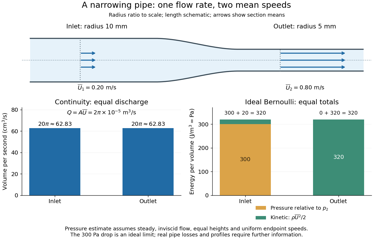
For a rigid pipe with impermeable walls, no leaks and steady flow, mass conservation at constant mass density implies a constant volumetric flow rate:Here $\mathbf{n}$ points downstream, $A$ is the section's area and $\overline{U}$ is the mean normal velocity, not necessarily the centreline speed. No assumption of inviscid flow or a uniform velocity profile is needed. If unequal amounts entered and left a fixed segment, its mass would accumulate, contradicting steady flow.

For a worked example, take horizontal water flow with stipulated mass density $1000\mathrm{kg}{\mathrm{m}}^{-3}$, inlet radius $R_1=0.010\mathrm{m}$, outlet radius $R_2=0.005\mathrm{m}$ and inlet mean velocity ${\overline{U}}_1=0.20\mathrm{m}{\mathrm{s}}^{-1}$. The circular areas giveThe radius halves, the area falls to one quarter, and the mean velocity quadruples. The mass flow rate is $\rho Q=0.02\pi \mathrm{kg}{\mathrm{s}}^{-1}$. The same amount of water passes both sections each second; narrowing changes its speed rather than compressing it. The Reynolds number and Bernoulli's principle discussions use this same example to examine viscous effects and the additional assumptions needed to calculate pressure.