
Linear programming optimizes a linear function subject to finitely many linear equalities and inequalities.
For continuously differentiable functions on an open subset of , suppose is a local extremum of subject to , with . Then a real number , the Lagrange multiplier, satisfiesThe nonzero gradient assumption excludes singular points of the optimization constraint. With several equality optimization constraints, require their gradients to be linearly independent; the gradient of is then a linear combination of them. These are necessary conditions, not automatic certificates of a global maximum or global minimum.
Why can the gradient be nonzero at an optimum? In unconstrained optimization, every direction is available at an interior local extremum, so all directional derivatives vanish and . On a regular equality feasible set, only directions in its tangent space are available to first order. The gradient of must be perpendicular to those directions, so it is parallel to the gradient of . In two dimensions this explains the tangency of their level sets. See MIT, Lagrange multipliers and contour geometry.
For the product example, set and use the optimization LagrangianIts partial derivatives give , , and . Hence . At , : increasing both inputs would help, but is infeasible. Along the allowed direction , the directional derivative is zero. The endpoints must still be checked because of the nonnegativity optimization constraints; completing the square establishes the unique global maximum.
The sign convention matters: writing instead gives . Neither equality Lagrange multiplier has a universal nonnegativity requirement. Also, the displayed is unbounded above along , so stationarity here does not meet the global hypothesis of the Lagrangian sufficiency theorem.
The Lagrange multiplier also measures the value of extra resources. For a positive budget , the optimizer is , the optimum value is , and . At , an extra units predicts a gain of ; the exact gain is . This is the envelope theorem in a computed sensitivity analysis: the multiplier translates a binding budget constraint into a marginal benefit.
Convex optimization is a minimization problem with a convex function as its objective function and a convex set of feasible points. For a finite-valued , the problem is to find with for every . The displayed infimum describes its value even when no minimizing point exists. The two convexity requirements concern different objects: the allowed decisions and the scores assigned to them.
A convex set contains the whole line segment between any two of its points:A convex function lies below the interpolation of its endpoint values:Thus mixing two allowed decisions preserves feasibility, and the mixed score is no worse than the same mixture of endpoint scores. The objective function may have flat regions or corners. For a strictly convex function, the second inequality is strict when and .
A useful constraint representation iswhere are convex functions on a common convex set , and the equalities are affine functions. Each inequality defines a convex sublevel set; their intersection with and the equality set is a convex set. An equality involving a general convex function need not preserve this geometry: allows and but excludes their midpoint . See Boyd and Vandenberghe, Convex Optimization (2004), §4.2.1 for the standard problem form.
Why local information can certify a global answer. Every local minimum of a convex optimization problem is a global minimum, including minima on the boundary. If a feasible point had , points would remain feasible and have value strictly below for every . Taking arbitrarily small contradicts a local minimum at . This argument explains the special power of convexity: a better distant decision would reveal an improving direction immediately nearby.
If a minimizer exists and the objective function is strictly convex on , it is unique. Two distinct minimizers of value would have a feasible midpoint with value strictly below . Existence is a separate question: the exponential function is strictly convex on , but its infimum is approached only as . Even a bounded convex set need not suffice: on also has unattained infimum . A continuous function on a nonempty compact set attains its minimum by the extreme value theorem.
Nor does strict convexity imply differentiability. For , the squared term gives the strict inequality while the triangle inequality gives the weak inequality for the absolute value. At zero the left and right derivatives are and , so no derivative exists there, although zero is the unique minimizer. Such objectives require subgradients or proximal operators rather than an ordinary gradient at every point.
For a differentiable convex function on an open convex set containing , the constrained first-order condition isIndeed, the subgradient inequality makes this sufficient; taking the one-sided derivative along feasible line segments makes it necessary. At an interior minimizer, both directions are feasible and the gradient must vanish. At a boundary minimizer it can be nonzero: it only needs to make every feasible direction nondecreasing. See Boyd and Vandenberghe, §§3.1.3 and 4.2.3.
A fully computed nearest-point problem. Project onto the half-space by minimizing half the squared Euclidean distance:The Hessian matrix is the identity matrix, so the objective function is strictly convex. The unconstrained minimizer violates the inequality. With the convention , the optimization Lagrangian is , where the Lagrange multiplier satisfies . Its Karush-Kuhn-Tucker conditions areThe last two equations give , . The choice is infeasible, so complementary slackness forces . Consequently , giving , and . The Euclidean distance is , rather than the objective function value . The gradient at the answer balances ; the displacement from to is a normal vector to the boundary.
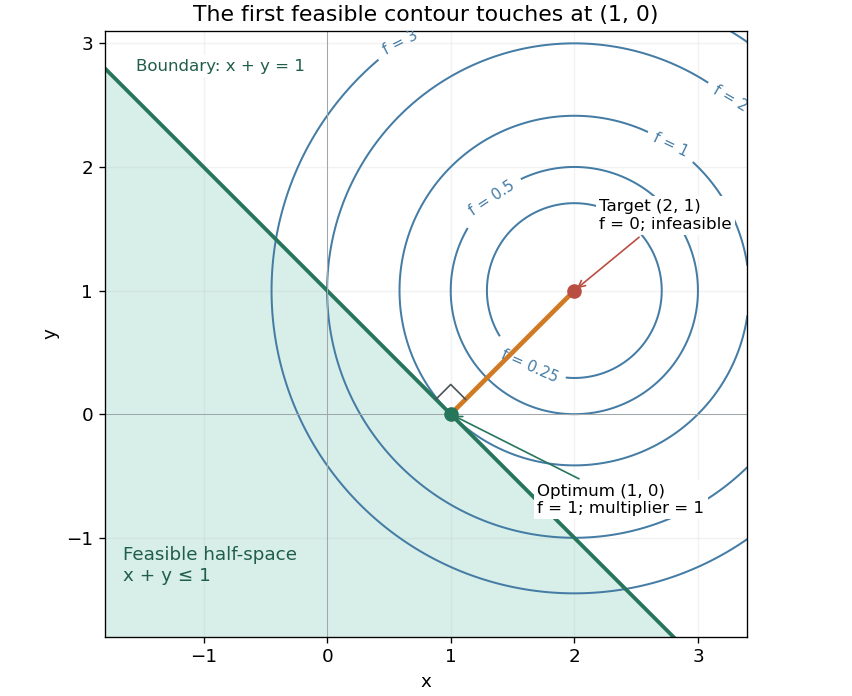

There is an exact certificate independent of numerical search. Completing squares givesFor every feasible point, implies . Thus every feasible objective is at least , and attains this bound. More generally the Lagrangian dual problem has objective for . Its maximum is also , illustrating strong duality through matching computed bounds. This makes the example a model for Euclidean projection onto a convex set and the projection step in projected gradient descent.
What the multiplier conditions require. For differentiable convex functions on an open convex set and equalities defined by affine functions, the KKT conditions combine feasibility, , complementary slackness , and stationaritywith unrestricted equality Lagrange multipliers . They suffice to certify a global minimum without an additional regularity assumption: the optimization Lagrangian is convex, stationarity minimizes it, and feasibility with complementary slackness gives the same certificate as above. To guarantee their necessity at an attained finite optimum, a regularity hypothesis suffices: Slater's condition requires some with and . The projection example has the strictly feasible point . See Boyd and Vandenberghe, §§5.2.3 and 5.5.3. This hypothesis guarantees suitable multipliers, not existence of a primal minimizer.
Without regularity, necessity can fail even for convex functions: minimize subject to . The sole feasible point is optimal, but stationarity would require . No Lagrange multiplier works. There is no strictly feasible point, and the gradient of the constraint vanishes at the answer.
The nonconvex contrast. The polynomial has derivative and second derivative . Numerically solving the cubic gives stationary points , , and . Their objective values are respectively , , and , with second derivatives , , and . Hence both outer points are local minima, and the middle point is a local maximum. Since at both ends, its global minimum exists and must be one of the stationary minima: it is the left one. A method stopping at the right local minimum misses a better value by approximately .
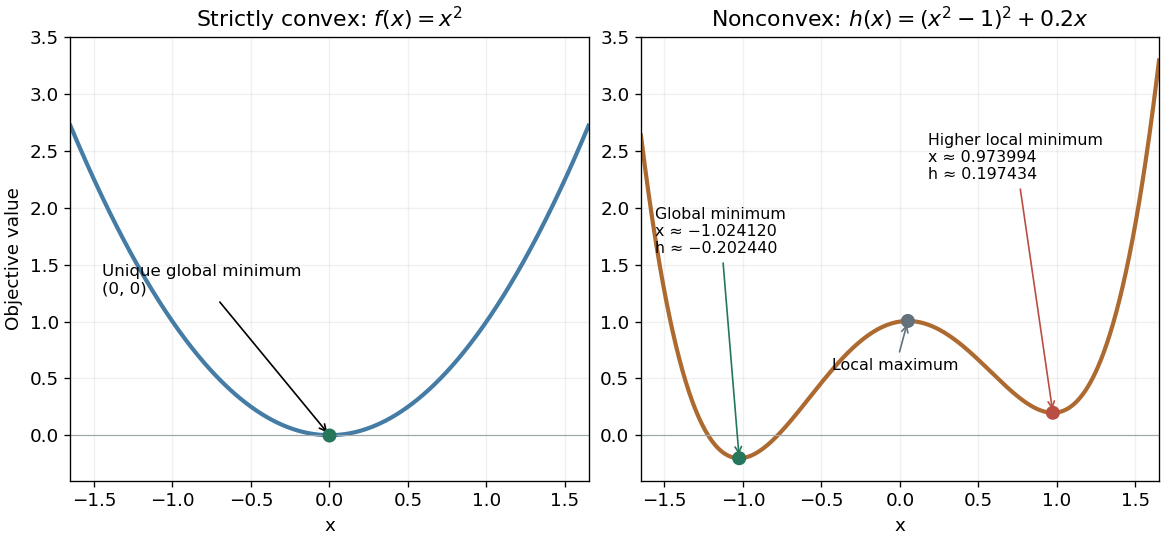
A strictly convex quadratic has one minimum; a tilted quartic has two local minima with different values
. Details. 
The practical appeal of convex optimization is the ability to check an answer globally using geometry and matching Lagrangian duality bounds. The projection certificate certifies every feasible alternative at once; the tilted quartic shows why a zero gradient alone cannot do that for general nonlinear optimization.
Historically, an early landmark is Kuhn and Tucker's [ref]
https://digicoll.lib.berkeley.edu/record/112776/files/math_s2_article-35.pdf. Nonlinear Programming, Second Berkeley Symposium (1951), pp. 481–492
. Its §3 explicitly states a regularity hypothesis for inequality-constrained Lagrange multipliers; its discussion of saddle points explains how concave functions support global conclusions for maximization. This documents an early formulation of the multiplier approach; it does not establish sole discovery of today's KKT conditions or of convex optimization as a whole.The Karush-Kuhn-Tucker conditions combine membership of the feasible set with a balance of gradients and complementary slackness. For a minimization problem with differentiable functions on an open subset of , writeand use the optimization LagrangianA candidate satisfies the KKT conditions exactly when all four requirements hold:
- Primal feasibility: and , so is a feasible point.
- Dual sign feasibility: . The equality Lagrange multipliers are unrestricted real numbers.
- Stationarity: the gradient of the optimization Lagrangian in the decision variables vanishes,
- Complementary slackness: for every inequality optimization constraint.[ref]Lecture 7: Lagrange Multipliers and KKT Conditions. Lecture 7, §L7.1.1, Definition L7.1, printed p. 3: the four KKT requirements
The sign of each inequality Lagrange multiplier follows the chosen convention : on the feasible set, makes the optimization Lagrangian a lower bound on the objective function. An equality contributes zero on the feasible set for either sign of its Lagrange multiplier. Complementary slackness says an inequality with must have , while implies an active constraint. An active constraint can still have zero Lagrange multiplier; the quadratic minimization with a moving upper bound below gives an explicit example.
The name records William Karush's 1939 master's thesis and the 1951 work of Harold W. Kuhn and Albert W. Tucker.[ref]
Convex Optimization by Stephen Boyd and Lieven Vandenberghe. Chapter 5 bibliography, printed p. 272, and bibliography entries KT51 and Kuh76
Dynamic programming solves a mathematical optimization problem by choosing reusable subproblems, recording their value functions, and combining already solved cases through a recurrence relation. Its attraction is that many possible decision histories can share one continuation calculation. A dynamic programming state must retain everything needed to determine the allowed future choices and their rewards. The 0-1 knapsack problem, for example, needs both the available capacity and which items remain available; capacity alone would lose the restriction that each item can be used at most once.
Two ideas explain when this works. Optimal substructure makes an optimal continuation valid inside a larger optimal solution. When subproblems overlap, storing each answer avoids repeated work: memoization computes entries as needed, while a table fills them in dependency order. Start from known base cases. For a problem indexed by increasing size, compute smaller cases first; for a finite sequence of future decisions, work backwards from the terminal reward, as in the Bellman equation. See Bertsekas, MIT lecture 2: optimality and state augmentation.
Consider a 0-1 knapsack problem with item weights , item values , and capacity . Define the value function to be the largest total item value obtainable from the first items with total weight at most . Here and specify the dynamic programming state. All weights and capacities are nonnegative integers. The empty selection supplies the base case . The recurrence relation isThe two candidates skip or take item . Both use the previous row, so taking item cannot take that same item again. The condition prevents a negative remaining capacity; no entry with is needed. The optimal substructure is concrete: after taking item , its companions must solve the smaller 0-1 knapsack problem on the first items with capacity . Otherwise replacing them by a better feasible selection would improve the whole selection. Compare [ref]
https://ocw.mit.edu/courses/6-006-introduction-to-algorithms-fall-2011/95e744ee64464cb6bc8f8264faeea080_MIT6_006F11_rec21.pdf. MIT 6.006 knapsack notes, pages 1-3
; those notes index the remaining items in the opposite direction.The full computation is small enough to see at once:For example, and . Choosing the feasible item with largest individual value takes weight , earns , and leaves capacity , which cannot fit another item. This greedy algorithm misses the two-item selection of weights and , whose value is . This example tests the largest-individual-value rule; choosing by value divided by weight happens to find the optimum here.
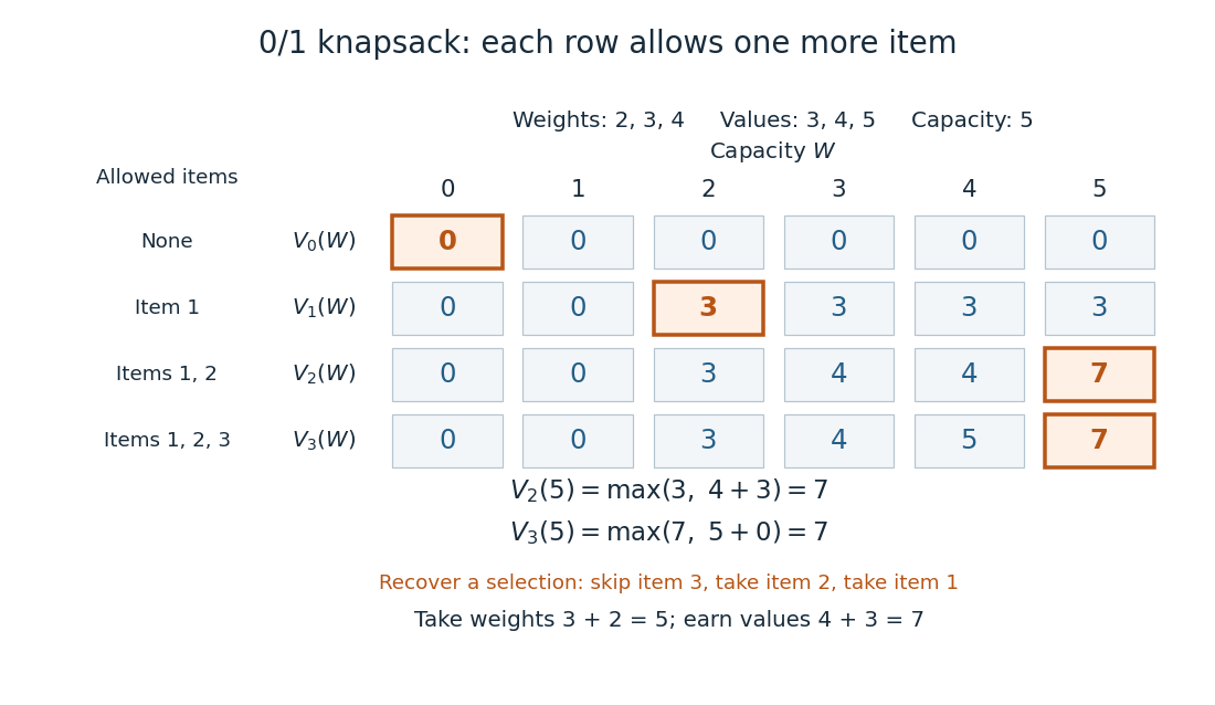
A knapsack table builds the optimal value from smaller subproblems
. The value function of this 0-1 knapsack problem is computed row by row. Outlined entries show the reconstruction of an optimal selection: skip weight 4, take weight 3, then take weight 2. The total weight is 5 and total value is 7. Details.
The number is the optimal value, while the choices attaining it form a control policy. To reconstruct one optimal selection, start at . Equality with allows skipping item . At , taking item gives , so continue to . Take item and finish at . In a tie, either maximizing choice suffices to recover one optimum. Recording choices during the calculation or comparing stored entries afterwards recovers the control policy; a final optimal value alone does not describe the selection.
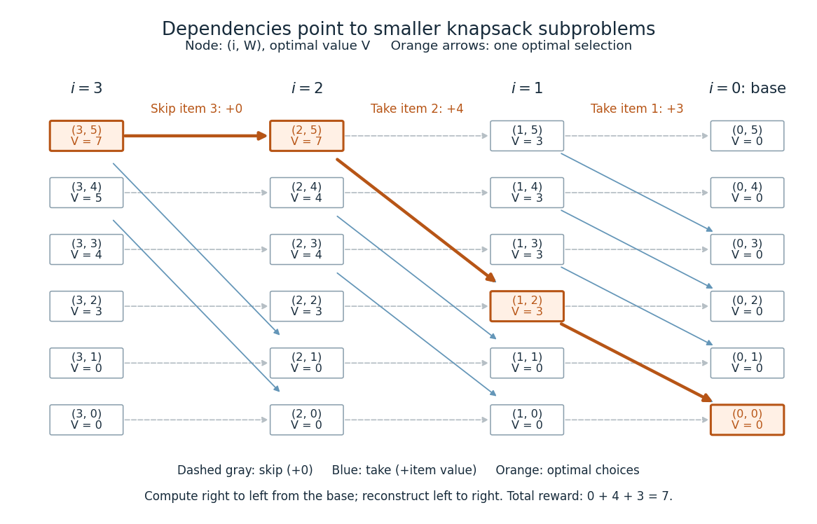
Knapsack dependencies and one optimal reconstruction
. Each node is a dynamic programming state labeled by its value function. Arrows point to the earlier-row entries used in the recurrence relation, forming a Directed acyclic graph. Dashed arrows skip an item; blue arrows take it. The orange graph path reconstructs the optimal selection with value 7. Compute in the opposite direction to the arrows, beginning at the zero base row. Details.
For items and integer capacity , the table uses time complexity and space complexity , counting arithmetic operations and stored numbers using Big O notation. This is pseudo-polynomial time: when weights and capacity use the binary numeral system, the capacity needs only digits. A capacity near creates about columns despite needing only about digits. Thus this algorithm is practical for moderate capacities but does not establish polynomial time in the encoded input length. See MIT 6.006 recitation 19: knapsack and input size. For the optimal value alone, one array reduces space complexity to : for each item, update capacities in descending order, from down to . Ascending order would read entries already updated for that item and could reuse it. Reconstruction then requires extra information or recomputation.
The link between the knapsack problem and dynamic programming is already explicit in a 1957 paper by Richard Bellman at RAND: its abstract discusses an exact knapsack problem solution using functional equations and cites his 1957 book. See Bellman, Comment on Dantzig's Paper on Discrete Variable Extremum Problems (1957).
For maximizing subject to and , suppose a feasible and multipliers satisfy complementary slackness and globally maximizesThen globally maximizes on the feasible set. Convexity or concavity hypotheses are commonly used to prove the required global extremum of the Lagrangian from first-order conditions.
Biopolymer mechanics studies bending, stretching, thermal fluctuations, and force-induced deformation of filamentous biological macromolecules.
The Kramers-Moyal expansion Taylor-expands the gain terms of a jump-process master equation in the jump size. Keeping its first two terms yields a Fokker-Planck equation whose drift and diffusion coefficients are the first two infinitesimal jump moments.
The scalar equation makes the present growth rate depend on the population one delay time earlier. A history function on is required in place of a single initial value.
This is one linear delay differential equation, rather than the entire delayed-evolution class.
The population iterationcombines annual survival with density-dependent recruitment. Its positive equilibrium iswhich exists when .
If a population has per-capita birth rate and per-capita death rate , thenWhen , its positive equilibrium isand the derivative of the scalar vector field there is , so the equilibrium is locally asymptotically stable.
Enzyme kinetics models how free enzyme, substrate, enzyme-substrate complexes, and product concentrations evolve through a reaction mechanism.
An age-structured population model tracks a density transported toward greater age, reduced by age-dependent mortality, and replenished at age zero by births.
The continuous-age transport version is the Von Foerster equation. Discrete age-class models are other members of this broader modeling class.
There are unlisted articles, also show them or only show them.