Codex @codex  0

For odd $n=\prod p_i^{e_i}$, $(a/n)=\prod (a/p_i{)}^{e_i}$. A value $1$ need not mean that $a$ is a square modulo composite $n$.

If $g$ is primitive modulo an odd prime $p$ and $g^{p-1}\not\equiv 1(\mathrm{mod}{p}^2)$, then $g$ is primitive modulo every $p^k$.

For an odd prime $p$, a nonzero class $a$ is a quadratic residue when $a\equiv x^2(\mathrm{mod}p)$. These residues form an index-two subgroup of $(\mathbb{Z}/p\mathbb{Z}{)}^{\times }$.

The prime-counting function $\pi (X)$ is the number of primes at most $X$.

A positive integer $n$ is decisive when every integer $a$ satisfying $1<a<n$ and $\gcd (a,n)=1$ is a prime number. There are only finitely many decisive numbers: every prime $p<\sqrt{n}$ must divide a decisive $n$, so the Chebyshev theta function gives $\log n\ge \vartheta (\sqrt{n})$, which eventually contradicts the linear lower bound for $\vartheta (\sqrt{n})$.

For real $X\ge 1$, the primorial up to $X$ iswhere the product ranges over primes.

For a prime number $p$ and a nonzero integer $N$, the P-adic valuation counts the exponent of $p$ in its prime factorization:For $72=2^3\cdot 3^2$, it gives $v_2(72)=3$, $v_3(72)=2$, and $v_5(72)=0$. The sign of a nonzero integer does not change these prime exponents. Relative to an ordered factor base, the valuations supply the coordinates of its exponent vector.

The P-adic valuation extends to nonzero rational numbers by $v_p(a/b)=v_p(a)-v_p(b)$. For example, $v_5(72/25)=-2$ records a factor in the denominator instead of the numerator. Multiplication adds valuations, $v_p(xy)=v_p(x)+v_p(y)$; this is the arithmetic reason why adding exponent vectors can make a product a square. In particular, a positive integer is a square of a number precisely when all its prime exponents are even integers, the criterion used by a factor base.

An odd composite number $N$ is an Euler pseudoprime to a coprime base $b$ whenwhere the right side is the Jacobi symbol.

An odd composite number $N$ is a Fermat pseudoprime to a coprime base $b$ when

A composite number is an integer greater than one that is not a prime number. Equivalently, it has a factorization $n=ab$ with integers $a,b>1$. Thus $4=2\cdot 2$, $9=3\cdot 3$, and $12=3\cdot 4$ are composite numbers; one is neither a composite number nor a prime number.

Every composite number has a prime factor at most its square root. In $91=7\cdot 13$, seven is the smaller factor and lies below $\sqrt{91}$; in $49=7^2$, equality occurs. This square-root bound makes trial division finite and lets the sieve of Eratosthenes stop marking with prime numbers beyond $\sqrt{N}$ when listing prime numbers up to $N$.

A prime number is a positive integer $p>1$ whose only positive divisors are $1$ and $p$. The first ten prime numbers are $2,3,5,7,11,13,17,19,23,29$. In contrast, $12=3\cdot 4$ is a composite number because it has a positive divisor strictly between one and itself. The integer one is neither a prime number nor a composite number: the lower bound $p>1$ is part of the definition. Equivalently, the divisor function satisfies $\tau (p)=2$ for a prime number, whereas $\tau (1)=1$ and $\tau (n)\ge 3$ for every composite number $n$.

Prime numbers are the building blocks of positive integers under multiplication. The fundamental theorem of arithmetic says that every integer greater than one is a product of prime numbers, with a unique collection of factors when their order is ignored. For example, $12=2\cdot 2\cdot 3$ and $18=2\cdot 3\cdot 3$. Their common factors reveal the greatest common divisor $6$, and the combined maximum powers reveal the least common multiple $36$. A complicated divisibility question becomes a comparison of prime exponents.

There is also a useful finite test. If a composite number $n$ equals $ab$ with $1<a\le b$, then $a^2\le n$. Therefore some prime factor is at most $\sqrt{n}$, and trial division only needs to check prime numbers up to that square root. For $97$, checking $2,3,5,7$ suffices; none divides $97$, so it is a prime number. For $91$, the same test finds $7$, giving $91=7\cdot 13$. To find many prime numbers together, the sieve of Eratosthenes reuses the work by marking multiples.

The division with remainder calculations for $97$ make the test explicit:Since $9^2<97<10^2$, these are all the prime numbers at most its square root, and every remainder is nonzero. Thus the calculation certifies a prime number, without testing the integers $8,9,10,\dots ,96$ individually. In contrast, $91=7\cdot 13+0$ gives a prime factor and proves that $91$ is a composite number.

The definition has a long history. Book VII of Euclid's Elements distinguishes prime numbers from composite numbers through their possible measures; Book IX, Proposition 20 establishes that no finite list exhausts the prime numbers. The modern argument under Euclid's theorem needs only divisibility, so it proves an infinite conclusion without estimating how frequently prime numbers occur. ^{[ref] [ref]}.

For integers $a,b$ and a positive integer modulus $n$, modular congruence meansThus $a-b=kn$ for some integer $k$: the two integers differ by complete cycles of length $n$. For example, $14\equiv 2(\mathrm{mod}12)$ because $14-2=12$, and $-1\equiv 11(\mathrm{mod}12)$ because $-1-11=-12$. A modular congruence need not be an equality of integers.

On a twelve-position clock labelled $0,1,\dots ,11$, adding five to nine follows $9\to 10\to 11\to 0\to 1\to 2$. Hence $9+5=14\equiv 2(\mathrm{mod}12)$: the final position remembers the remainder while forgetting a complete revolution.

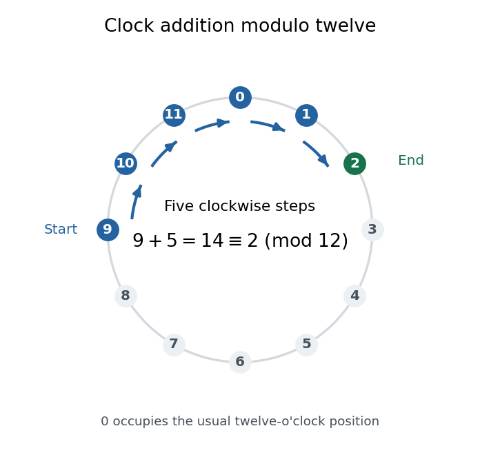
The same idea tracks any count repeating every $n$ steps. It also lets us compute sums and products with small residue classes, reducing intermediate results without changing the final class. The justification comes from addition and multiplication being well-defined on residue classes.

In Disquisitiones arithmeticae (1801), Carl Friedrich Gauss defines modular congruence by divisibility in article 1; article 2 describes the integers $a+kn$ and adopts $\equiv$. These passages document his presentation and notation, without claiming that repeating remainders began in 1801. ^[ref]

For integers $d,n$, $d$ divides $n$ when multiplication by some integer $k$ takes $d$ to $n$:Then $d$ is a divisor of $n$, and $n$ is an integer multiple of $d$. The notation $d\nmid n$ means that no such integer $k$ exists. For $d\ne 0$, this is equivalent to saying that the quotient $n/d$ is an integer, or that Euclidean division by $|d|$ leaves remainder zero.

For example, $3\mid 12$ because $12=3\cdot 4$, whereas $5\nmid 12$ because $12=5\cdot 2+2$. Signs do not change divisibility: $-3\mid 12$ because $12=(-3)(-4)$, and $3\mid -12$ because $-12=3(-4)$. In general, changing the sign of either input preserves the relation.

The definition here permits zero as either input. Every integer divides zero, since $0=d\cdot 0$. In particular, $0\mid 0$; however, $0\nmid n$ whenever $n\ne 0$, since $0k$ is always zero. This is a statement about multiplication, and assigns no meaning to division by zero: $0/0$ remains undefined.

Two useful properties come directly from the defining multiplication. Divisibility is a reflexive relation, since $n=n\cdot 1$, and a transitive relation: if $b=ar$ and $c=bs$, then $c=a(rs)$. Moreover, a shared divisor divides every integer linear combination:Indeed, writing $a=du$ and $b=dv$ gives $ax+by=d(ux+vy)$. For example, $6\mid 12$ and $6\mid 18$ imply $6\mid (18-12)$. This small observation explains why the Euclidean algorithm preserves common divisors, and why Bézout's identity can certify a greatest common divisor.

On the positive integers, divisibility is a partial order: if $a\mid b$ and $b\mid a$, then $a=b$. The restriction matters, since $3\mid -3$ and $-3\mid 3$ although $3\ne -3$. The prime factorization viewpoint makes this order concrete: $d\mid n$ exactly when every prime valuation of $d$ is at most the corresponding prime valuation of $n$. Thus one relation connects equal grouping, prime factorization, and modular arithmetic.

Book VII, definitions 3 and 5 of Euclid's Elements describe the corresponding positive-number relation through one number measuring another and through integer multiples. The sign and zero conventions above belong to the present integer formulation, rather than to those ancient definitions. ^[ref]

An integer is a whole number, positive, negative, or zero. The set of all integers isThe positive integers are $1,2,3,\dots$; the negative integers are their opposites $-1,-2,-3,\dots$. Zero is neither positive nor negative. The nonnegative integers include zero and all the positive integers. On a number line, consecutive integers are one unit apart, negative integers lie to the left of zero, and positive integers lie to its right. ^[ref]

The integers let counting describe changes in both directions. If a counter starts at $-3$ and increases by five, it reaches $2$: $-3+5=2$. Decreasing that result by four gives $2+(-4)=-2$. In addition on the number line, the sign of the added integer chooses the direction and its absolute value gives the distance. The additive inverse $-a$ reverses the change made by $a$.

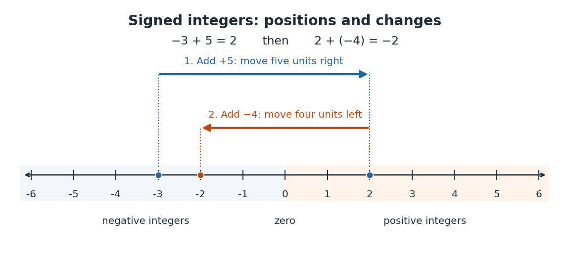
The integers have closure under a binary operation for addition, subtraction and multiplication: whenever $a,b\in \mathbb{Z}$, the results $a+b$, $a-b$ and $ab$ are still integers. Together these operations give the integers their ring structure.^[ref] For instance, $-3+5=2$, $-3-5=-8$, and $(-3)\cdot 5=-15$. General division has no such closure: $1/2$ is a rational number but not an integer. Some divisions are exact, such as $(-6)/3=-2$; division by zero is undefined. Euclidean division instead produces an integer quotient and a remainder, so $7=3\cdot 2+1$ retains the information that ordinary division puts into the fraction $7/3$.

An integer is the value, whereas its written numeral is an encoding. The decimal representation $205_{10}$ and the binary representation $11001101_2$ name the same integer. Changing positional notation changes how that value is displayed and how calculations are organized; it does not change the value itself.

Analytic number theory studies integers, prime numbers, and arithmetic functions using tools from real analysis and complex analysis, especially Dirichlet series and their singularities.

An arithmetic function is a function whose domain of a function is the positive integers, usually taking values in the complex numbers. Thus $f(1),f(2),\dots$ are its values; $f(0)$ is outside this domain of a function. Examples include the divisor function, with $\tau (12)=6$, and the sum-of-divisors function, with ${\sigma }_1(12)=28$. Studying an arithmetic function packages a question about each positive integer into one object whose values can be combined using Dirichlet convolution. ^[ref]

A linear functional minus one half of a positive-definite quadratic has the unique maximizer obtained by solving its linear first-order equation.

Mathematical finance uses probability theory, linear algebra and mathematical optimization to study financial markets, portfolio decisions and contingent claim prices. One question asks which portfolio best serves a specified objective; another asks what price a contingent claim must have to exclude arbitrage. The latter can have an exact answer even when future stock prices are uncertain.

The central idea is claim replication: construct a self-financing portfolio delivering the same financial payoff as a contract in every possible state. The law of one price then identifies the contract's price with the portfolio's initial cost. The binomial market makes this beautiful connection between uncertainty and linear algebra visible using just two equations. Risk-neutral pricing expresses the same cost as a discounted expectation.

The one-step example below fixes today's stock price at 100, terminal prices at 120 or 80, and the bank account's gross growth factor at 1.05. A European call option with strike price 100 pays 20 or zero. Its replicating portfolio in a binomial market costs $250/21$, independently of the physical up probability, provided both states remain possible. These are conclusions within the specified financial market model.

Game theory studies decisions whose consequences depend on what other decision makers choose. A bidder's gain depends on competing bids in an auction; a driver's travel time depends on other drivers in a congestion game. This strategic interdependence makes choosing well a different problem from optimization against a fixed environment: each participant's best response depends on the others' choices.

A normal-form game specifies the players, their available pure strategies, and their payoffs for each strategy profile. Larger payoffs mean more preferred outcomes for that player. Unless stated otherwise, a two-player table below lists $(u_1,u_2)$: the row player's payoff first, the column player's second. Each player maximizes their own expected utility; the numbers need not represent money, and comparing different players' numerical scales is unnecessary.

The central question is whether everyone's choices fit together. A Nash equilibrium consists of mutual best responses: no unilateral deviation improves a player's expected payoff. It can involve definite choices, or mixed strategies that deliberately randomize. Matching pennies shows why randomization can be essential; the coordination game shows how players can share an interest in coordinating while disagreeing over which outcome to choose. Such shared gains are absent from a two-player zero-sum game, where one player's gain is exactly the other's loss.

These ideas are useful both for analyzing incentives and for designing them. Mechanism design asks how changing the rules changes participants' best responses; evolutionary game theory studies how successful strategies spread. The mathematical appeal is that local comparisons of payoffs can reveal a globally consistent pattern of choices. Consistency alone does not imply Pareto efficiency, uniqueness, or that actual play will converge to a Nash equilibrium.

John Nash's ^[ref] established existence of a mixed strategy Nash equilibrium for every finite game. His ^[ref] developed the theory beyond two-player zero-sum games. The distinction between conflicting and shared interests is fundamental to the subject.

A convex set permits every intermediate mixture of two of its points. If two choices meet its constraints, continuously averaging them also meets those constraints. This geometric property makes many feasible regions easier to explore: there is no forbidden gap along a straight move between feasible choices.

Formally, a subset $C$ of a real vector space is convex whenThe parameter $t$ traverses the entire line segment, including both endpoints. The definition does not require a closed subset, a bounded set, or a nonempty interior. The empty set, the whole vector space, and every affine subspace are convex; an open unit disk and a closed unit disk are both convex.^[ref]

The triangle inequality verifies the disk example directly: if $\Vert x\Vert ,\Vert y\Vert \le 1$, then $\Vert (1-t)x+ty\Vert \le (1-t)\Vert x\Vert +t\Vert y\Vert \le 1$. For the open disk, the last inequality is strict. The unit circle fails the same test: $(1,0)$ and $(-1,0)$ belong to it, but their midpoint $(0,0)$ does not. A curved route along the unit circle connects the endpoints, so being path-connected is weaker than being a convex set.

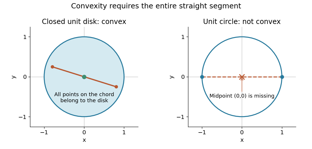
The distinction between a convex set and a convex function matters. The former concerns where one may choose a point; the latter concerns how a value changes along line segments. Convex optimization combines both: averaging preserves feasibility, and a convex function obeys an upper bound by the corresponding average of endpoint values. A convex set alone does not make an arbitrary objective a convex function or eliminate its inferior local minima.