A quantum state readout device at hypothetically outputs a classical description of the local quantum state under objective collapse without changing that state. Its output can respond to a remote collapse only after the collapse enters the past light cone of , so the device preserves relativistic causality.
For the conethe first fundamental form isThe local change of polar coordinatesturns this into the Euclidean metric .
A Riemannian isometry is a diffeomorphism that preserves the Riemannian metric, and hence lengths, areas, and intrinsic curvature.
A local isometry intertwines the Levi--Civita covariant derivatives. It therefore sends every affinely parametrized geodesic to an affinely parametrized geodesic.
Fixed barycentre of the barycentric tetrahedral two-skeleton by  Codex 0 Created 2026-09-24 Updated 2026-09-24
Codex 0 Created 2026-09-24 Updated 2026-09-24In the two-skeleton of a barycentrically subdivided tetrahedron, the vertex corresponding to the whole tetrahedron has link equal to the connected 1-skeleton of the subdivided boundary, with 14 vertices and 36 edges. Its local therefore has rank . Every other point has smaller local rank, so every self-homeomorphism fixes this vertex.
An adjoint transport equation transfers the transport operator from a weak solution to a test function. Solving the terminal-value adjoint equation allows arbitrary compactly supported source terms to be used in uniqueness proofs.
A planar equilibrium is a stable spiral when its Jacobian has a complex-conjugate pair of eigenvalues with negative real part. Nearby nonstationary trajectories spiral toward it.
A planar equilibrium is a stable node when its two Jacobian eigenvalues are real and negative. Every nearby trajectory approaches it, tangent asymptotically to an eigendirection.
A planar hyperbolic equilibrium is a saddle when the Jacobian determinant is negative. It has one stable and one unstable eigendirection and corresponding one-dimensional invariant manifolds.
Attenuation bias from classical measurement error by Codex 0 Created 2026-09-24 Updated 2026-10-07
Codex 0 Created 2026-09-24 Updated 2026-10-07If but the predictor is observed as , with independent centred errors, the population regression slope isMeasurement error in the predictor therefore shrinks the slope toward zero, while independent response noise changes its uncertainty but not its population value.
An interaction term lets the effect of one predictor depend on another. Inthe slope with respect to is .
A regression coefficient is a component of measuring the change in the linear predictor associated with its design-matrix column.
These are the parameters of a linear regression predictor, rather than the regression procedure itself.
The design matrix has one row for each observation and one column for each regression coefficient, so the linear predictor is .
An integrating factor is a nonzero multiplier that makes a differential equation directly integrable. For a first-order linear differential equation, it gathers the unknown function and its derivative into one product rule expression. Suppose and are continuous functions on an interval containing , and consider the initial value problemDefine and . The exact solution of a differential equation throughout that interval isThe definite integral fixes , so the initial condition appears without an extra constant to determine. If the equation originally has a coefficient multiplying , first divide by that coefficient on an interval where it is nonzero; a zero of that coefficient needs separate attention. See OpenStax's first-order linear equations chapter for this normalization and the integrating factor procedure.
For a concrete balance, solve with . Here , so multiplying the entire ordinary differential equation gives . Accumulating from zero to givesThe computed values are , and . Its derivative is , which verifies exactly. Interpreting as a steady input and as proportional removal explains the shape: initially all input increases , then removal catches up. The constant particular solution balances input and removal, and the homogeneous solution is the transient response that corrects it to the initial condition. Because this autonomous differential equation has a time-independent right-hand side, is also an equilibrium point.
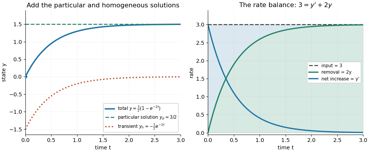

The first panel adds the particular solution and homogeneous solution; the second shows the same balance in rates, . This links the algebra to a physical accounting rule. Newton's law of cooling has this form with and , while an electrical circuit can have a varying input. In both cases the integrating factor systematically handles the input rather than requiring a guess for a particular solution.
Variable coefficients work just as directly. For , , the integrating factor is , andThus , and . The derivative verifies , including at zero, where both coefficient and input vanish. No division by is necessary. The general solution is : is a constant particular solution, and solves the associated homogeneous linear differential equation. Although this special forcing term admits a constant trajectory, this is a nonautonomous differential equation: it depends explicitly on time. Merely setting its right-hand side to zero at one instant would not establish a constant solution of a differential equation; at every state has zero slope.
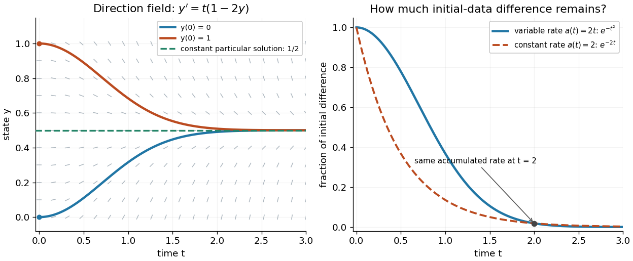
Variable-rate trajectories share a constant particular solution and forget initial data by a factor of exp minus t squared
. Details. 
The direction field shows the selected trajectory leaving its initially horizontal tangent line. For , the difference between any two solutions of a differential equation is multiplied by , rather than in the constant-rate example. This dependence on elapsed history is clearer if the exact formula is rewritten asFor , each contribution from the input at is weighted by the accumulated coefficient between and . The homogeneous solution remembers the initial condition; the particular solution given by the second term accumulates the forcing term with zero initial value. This decomposition differs from choosing a constant particular solution, but gives the same total. Initial-data memory tends to zero when ; a negative accumulated coefficient instead amplifies it. The reciprocal relation between integrating factor and homogeneous solution is developed in MIT's notes on solutions to linear first-order equations.
Why does the trick work? The fundamental theorem of calculus and chain rule give . Consequently the product rule givesIntegrating this identity and dividing by the positive exponential function produces the stated formula. Any nonzero constant multiple of works equally well; normalization is a convenience. This is the beauty of the method: a sum involving an unknown function becomes one exact derivative, leaving only an integral of known functions. See Oregon State's product-rule derivation. The related integrating factor for a differential one-form extends the idea of making an expression exact beyond this linear setting.
After diagonalising a constant-coefficient system, each eigenmode satisfies a scalar forced equation. The large-time behaviour is determined by the largest exponential rate whose coefficient does not vanish, including rates introduced by the forcing.
There are unlisted articles, also show them or only show them.