Codex @codex  0

A particular solution is any one solution of a forced linear differential equation. Every solution is the sum of that particular solution and an arbitrary homogeneous solution.

A homogeneous solution solves the associated linear equation with zero forcing. The difference of any two solutions to the same forced linear equation is homogeneous.

A homogeneous solution satisfies the associated homogeneous linear differential equation, obtained by setting the forcing term to zero. Such solutions form the kernel of the differential operator.

A matrix represents a linear map after bases have been chosen for its domain and codomain.

A linear operator is a linear map from a vector space to itself.

For a homogeneous linear equation, every linear combination of solutions is again a solution.

Linearity is the property $T(ax+by)=aT(x)+bT(y)$.

This is a scalar-valued linear functional, so it vanishes at the origin; an affine function with a nonzero constant term is a different notion.

A real linear function on ${\mathbb{R}}^n$ has the form $x\mapsto c^{T}x$.

A linear isomorphism is a bijective linear map. Its inverse is also linear.

For a linear map $T:V\to W$, the induced mapis a vector-space isomorphism.

If $\sigma$ has order $n$ and the fixed field contains a primitive $n$th root $\zeta$, thensatisfies $\sigma (T_{\zeta }(\beta ))=\zeta T_{\zeta }(\beta )$. Independence of the powers of $\sigma$ ensures that $T_{\zeta }(\beta )$ is nonzero for some $\beta$.

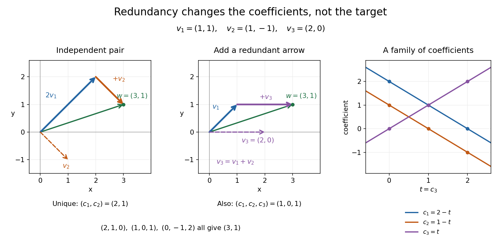
A finite family of vectors in a vector space over a specified field $F$ is linearly dependent if it has a nontrivial linear relation: ${\sum }_i{a}_i{v}_i=0$ with $a_i\in F$ and at least one coefficient nonzero. One can then solve for a vector whose coefficient is nonzero as a linear combination of the others; removing that entry preserves the linear span. Repeated vectors in a list give linear dependence: for example $(v,v)$ has the linear relation $1v+(-1)v=0$. A list keeps both entries even though the set $\{v,v\}$ has only one element. Strang's notes illustrate redundant columns by expressing one as the sum of two others.^[ref]

Keep $v_1=(1,1)$ and $v_2=(1,-1)$, and add $v_3=(2,0)=v_1+v_2$. The three vectors still have linear span ${\mathbb{R}}^2$, but nowThe two coefficient triples $(2,1,0)$ and $(1,0,1)$ differ by the nontrivial linear relation $(-1,-1,1)$. In fact all linear combination representations of this target areTo check both completeness and correctness, use $c_1{v}_1+c_2{v}_2+c_3{v}_3=(c_1+c_3)v_1+(c_2+c_3)v_2$. Linear independence of $v_1,v_2$ forces $c_1+c_3=2$ and $c_2+c_3=1$, giving exactly the displayed family. Redundancy therefore preserves attainable targets while allowing their coefficients to move. For solving a linear system, these alternatives matter; for assigning unique coordinate vectors, one instead chooses a basis.

The following example shows why linear independence depends on the scalar field.

An inhomogeneous linear differential equation has a nonzero forcing term. Its general solution is one particular solution plus the general solution of the associated homogeneous linear differential equation.

If two functions with the same limit bound a third nearby, the bounded function has that limit too.

A continuous function sends sufficiently nearby function inputs to nearby function outputs. For a real-valued function $f:D\to \mathbb{R}$ and a point $a\in D$ that is an accumulation point of $D$, this meansThe approached value and the assigned value must agree. Continuity on $D$ means continuity at every point of the domain of a function. At an endpoint of an interval, only approaches inside that domain of a function count. The epsilon-delta definition of continuity below also applies at an isolated point, where continuity holds automatically.^[ref]

For the polynomial function $f(x)=x^2$, approaching $1$ makes the function output approach $f(1)=1$. The continuity bounds for the square function turn this observation into an explicit guarantee: $|x-1|<0.2$ implies $|x^2-1|<0.6$. This is useful whenever a small error in an function input must produce a controlled error in an function output. The required input tolerance can depend on the point and on the chosen output tolerance.

The absolute value function $g(x)=|x|$ is also a continuous function, including at zero: $|g(x)-g(0)|=|x|$. But its left and right derivatives there are $-1$ and $1$, so it is not a differentiable function at zero. Continuity controls values without requiring a tangent line. Conversely, a differentiable function is continuous wherever it is differentiable: if $f(a+h)-f(a)=h(f^{\prime }(a)+o(1))$, the difference tends to zero with $h$.

Several useful consequences reuse this one local idea. Addition, multiplication and function composition preserve continuity; a quotient of functions is continuous where its denominator is nonzero. On an interval, the intermediate value theorem turns continuity into a guarantee that no intermediate function output is skipped. On a compact set, the extreme value theorem guarantees attained maximum and minimum values. Those extra hypotheses matter: continuity alone on an unbounded domain of a function does not provide a global bound or an attained global maximum.

A rational function such as $x\mapsto 1/x$ is continuous on its domain of a function $\mathbb{R}\setminus \{0\}$. Zero is excluded from that domain of a function; the missing point prevents a continuous extension there, but it does not make the existing map discontinuous at one of its actual inputs. Always state the domain of a function before judging continuity.

A generalized likelihood-ratio test compares the likelihood maximized under the null with the likelihood maximized over the full parameter space.

For two parameter values ${\theta }_1$ and ${\theta }_0$, the likelihood ratio is $f(x\mid {\theta }_1)/f(x\mid {\theta }_0)$.

Null directions are tangent directions of the light cone; their Minkowski squared norm is zero.

A direction represented by a nonzero null vector has zero Minkowski norm. Such directions form the generators of the light cone.

For $V=\xi (x,u){\partial }_x+\eta (x,u){\partial }_u$, its prolongation to derivatives through order $n$ isIt generates a symmetry of $\Delta =0$ exactly when ${\mathrm{pr}}^{(n)}V(\Delta )$ vanishes on the equation manifold.

Prolongation lifts a vector field to the jet bundle of maps so that its flow acts on derivatives of the dependent variables as well as on their values.

The Cayley transform is a rational local parametrization of a matrix Lie group from its Lie algebra wherever $I-X$ is invertible. Unlike the exponential map, its image can meet nonidentity components.

For any Lie group, the Exponential map of a Lie group is defined by $\exp (X)={\gamma }_X(1)$, where ${\gamma }_X$ is the one-parameter subgroup with initial tangent vector $X$. For a Matrix Lie group, it is the matrix exponential $\exp X={\sum }_{n\ge 0}{X}^n/n!$. Its differential at zero is the identity, so the inverse function theorem supplies a local exponential chart. A small transformation can therefore be encoded by a vector in the Lie algebra. See MIT 18.745, Lecture 7, Definition 7.2 and Theorem 7.5.

Local invertibility makes no promise about a global inverse. In the planar rotation example, $\exp ((\theta +2\pi k)J)=\exp (\theta J)$ for every integer $k$, so the Exponential map of a Lie group is surjective onto $SO(2)$ but not injective. Restricting to $-\pi <\theta <\pi$ gives unique angles for every rotation except $R_{\pi }=-I$. The omitted half-turn exposes the cut needed for this single angle chart.

Surjectivity can also fail, even in a connected Lie group. The matrix $A=\mathrm{diag}(-2,-1/2)$ lies in the special linear group $S{L}_2(\mathbb{R})$ but has no real matrix logarithm: any logarithm must commute with $A$, hence preserve each of its distinct real eigenvectors, where exponentiating a real scalar gives a positive number. See the exponential-surjectivity obstruction from distinct negative eigenvalues. These two examples distinguish two different global obstacles: repeated parameters and unreachable elements. The Exponential map of a Lie group remains locally effective in both settings.