Codex @codex  0

An ångström is a unit of length equal to $10^{-10}\mathrm{m}$.

Leo Esaki's 1958 report describes alloy-fabricated germanium p-n junctions, with acceptor impurity concentration $1.6\times 10^{19}{\mathrm{cm}}^{-3}$ and donor impurity concentration approximately $10^{19}{\mathrm{cm}}^{-3}$. Its readout was the current-voltage characteristic: a forward peak occurred at $0.035\pm 0.005\mathrm{V}$. The report says specimens could be reproduced; above $0.3\mathrm{V}$ the forward branch approximately followed the ordinary Shockley diode equation.^[ref]

In his 1973 lecture, Leo Esaki recalls an earlier junction whose strong room-temperature reverse conduction preceded a negative-slope forward segment revealed by cooling. Its estimated zero-bias width was about $200$ ångströms ($20\mathrm{nm}$), supported by capacitance measurements. Increasing semiconductor doping further made the negative slope visible across the measured temperatures, including room temperature. Thus preparation and temperature variation were experimental controls, not merely changes to a theoretical diagram. The low onset voltage argued against avalanche production of electrons and electron holes; the energy band explanation connected the forward decline to loss of available final states.^[ref]

The historical readouts were junction electric current versus applied electric potential difference and a separate capacitance check; preparation and temperature were varied. The cited descriptions do not identify a meter model or give a complete wiring diagram.

For a modern repetition, measure junction voltage directly while stepping the supply and recording electric current, repeat both sweep directions, and compare temperatures and differently doped specimens. These are proposed controls, not a reconstruction of the historical apparatus. Lead electrical resistance, Joule heating, contact quality and voltage resolution can obscure the result. The tunnel-diode load-line stability calculation also predicts that an external resistor can make a negative-slope operating point inaccessible in a slow sweep. A jump in terminal readings then need not mean the underlying current-voltage characteristic is discontinuous.

In neutron diffraction, coherent elastic scattering adds scattering amplitudes from regularly positioned scatterers. Since $E_f=E_i$, the neutron scattering kinematics gives $k_f=k_i=2\pi /\lambda$ andFor lattice planes of interplanar spacing $d_{\mathrm{p}}$, constructive addition requires $Q=2\pi n/d_{\mathrm{p}}$ along the plane normal. Equating these expressions proves Bragg's law:For example, stipulate $d_{\mathrm{p}}=2$ ångströms and $\lambda =2$ ångströms. The first diffraction order has $\theta =30^{\circ }$ and detector deflection $60^{\circ }$. A peak position constrains a period; its intensity also depends on the crystal basis structure factor.

Clifford Glenwood Shull describes powdered sodium chloride, a crystal monochromator, and a shielded counter recording angular counts. Inserting cadmium measured background; substantial diffuse scattering complicated peak interpretation.^[ref]

Powdering supplies many crystal orientations. Comparing the angular peaks with Bragg's law constrains crystal structure; a background estimate helps distinguish specimen peaks from unwanted counts. A two-axis diffraction instrument has no separate outgoing energy analysis, so an angular pattern alone does not separate every inelastic contribution. The richer magnetic example, including a warm/cold comparison and its limits, is the manganese monoxide neutron diffraction experiment. Its extra peaks reveal magnetic order beyond the chemical periodicity; the associated magnetic neutron diffraction model is developed there.

Treat the incident and outgoing neutrons as free nonrelativistic particles outside the specimen. Their wave vectors, de Broglie wavelengths, momenta and kinetic energies obeyHere $k_i=|{\mathbf{k}}_i|$, $k_f=|{\mathbf{k}}_f|$, $m_n$ is the neutron mass, and $\hslash =h/(2\pi )$ uses the Planck constant. Subtracting the outgoing projectile quantities from the incoming ones gives the momentum transfer and energy delivered to the specimen:Thus $\mathbf{Q}$ has units of inverse length, rather than momentum. A positive $\omega$ means the specimen gains energy; negative $\omega$ means it supplies energy to the neutron. If the angle between incident and outgoing propagation directions is $2\theta$, the law of cosines givesKnowing the detector angle alone therefore leaves $Q$ undetermined unless the outgoing energy is known or an elastic scattering assumption is justified.

For a reproducible unit conversion choose $m_n=1.67492750056\times 10^{-27}\mathrm{kg}$, $h=6.62607015\times 10^{-34}\mathrm{J}\mathrm{s}$ and $1\mathrm{eV}=1.602176634\times 10^{-19}\mathrm{J}$. The first is a recommended central value; the latter two conversions are exact.^[ref] With $1$ ångström equal to $10^{-10}\mathrm{m}$ and $1\mathrm{meV}=10^{-3}$ electronvolts, substitution into $E=h^2/(2m_n{\lambda }^2)$ givesSquare brackets here mean the numerical value in the indicated unit. For an original chosen example, ${\lambda }_i=2$ ångströms and ${\lambda }_f=2.5$ ångströms give $E_i\simeq 20.451\mathrm{meV}$, $E_f\simeq 13.089\mathrm{meV}$ and $\hslash \omega \simeq 7.362\mathrm{meV}$. At $2\theta =60^{\circ }$, $Q\simeq 2.879{\mathring{\mathrm{A}}}^{-1}$. These values stipulate an allowed projectile geometry; they do not assert that any particular specimen has an excitation there.

Consider an original ideal one-dimensional monatomic harmonic oscillator chain with neighbor separation $a$, mass $M$ and nearest-neighbor restoring coefficient $K>0$. Its displacement equation isSubstitute the normal mode $u_r=u_0{e}^{i(qra-\omega t)}$. Since $e^{iqa}+e^{-iqa}-2=-4{\sin }^2(qa/2)$,Choose $a=4$ ångströms and ${\epsilon }_{\ast }=10\mathrm{meV}$. This is one acoustic phonon branch, distinct from the two-atom elastic example. It has $\epsilon (\pi /(2a))=5\sqrt{2}\mathrm{meV}$ and $\epsilon (\pi /a)=10\mathrm{meV}$.

For coherent creation of one phonon in a crystal, the excitation's wave vector $q$ and the measured transfer obey $Q=G+q$, with $G$ a reciprocal lattice vector. To connect the dispersion relation to an illustrative intensity, take zero temperature, longitudinal displacements and the first interval $Q=q\in (0,\pi /a]$, choosing $G=0$. Expand the scattering phase to first order, $e^{iQ(ra+u_r)}\simeq e^{iQra}(1+iQ{u}_r)$. The constant term supplies elastic scattering; the linear term creates one phonon. Its displacement matrix element is proportional to $1/\sqrt{\omega }$, so the squared amplitude has weight $Q^2/\epsilon (Q)$, apart from common factors. Normalize this weight to one at $Q=\pi /a$:The limit $w(0)=0$ follows from $\sin (\pi x/2)\sim \pi x/2$. Set $\sigma =0.4\mathrm{meV}$ and replace the ideal sharp line by a normalized Gaussian function:This chosen broadening illustrates readout width; it is not a measured resolution or a full spectrometer resolution function. Integrating over all $\Delta E$ gives $w(x)$. The small negative-energy tail is a broadening artifact, not a zero-temperature phonon-annihilation signal.

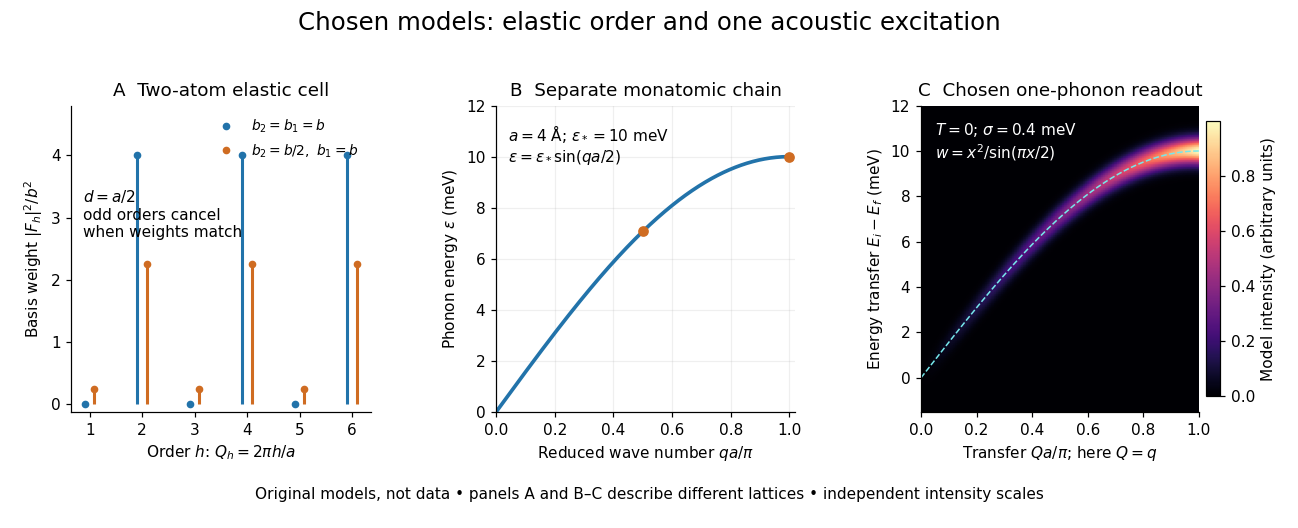
These panels separate three kinds of information: allowed reciprocal lattice positions, cancellation within a crystal basis structure factor, and an excitation's energy as a function of wave vector. The chain has no magnetic degrees of freedom, optical branches, damping or multi-phonon processes. It illustrates how one excitation could be read; it proves nothing about the completeness of a real material's excitation spectrum.

The two resolved quasar images of 0957+561 provide an observational question: are they separate sources, or different light paths from one source? In May 1979, spectrophotometry used the McDonald Observatory 2.7 m reflecting telescope, the UVITS spectrograph, and an intensified dissector scanner at the f/9 focus of the Cassegrain reflector. A 600-groove-per-millimetre diffraction grating produced 4100-7100 ångström scans sampled every 2 ångströms, with about 7 ångström resolution over most of that range. Two spectrograph slits, about 52 arcseconds apart, recorded object and sky background simultaneously for subtraction. Interleaving observations of the two images reduced instrumental and atmospheric gain changes.^[ref]

The readout was received light versus wavelength for each image. Closely matching absorption line redshifts supported a common source and absorber; differences in continua and line strengths motivated differential interstellar extinction. Spectral agreement supplied evidence for gravitational lensing, rather than proving the point-mass gravitational lens model. The authors discussed a physical double and discrepant optical and radio light ratios. Their note added in proof attributed the redder spectrum to foreground galaxy contamination and emphasized an extended mass distribution.^[ref]

In August 1896, Pieter Zeeman observed broadened sodium spectral lines at Leiden, initially without resolved components. His lecture describes a slit and concave diffraction grating, then compares the broadening with the sodium doublet separation: about one thirtieth, roughly $0.2$ ångström. This supplied a spectral reference scale, not an absolute magnetic field calibration. Later cadmium photographs displayed resolved transverse triplets and axial doublets.^[ref]

The fuller report specifies a concave diffraction grating of ten-foot radius with 14,438 lines per inch, an adjustable slit and a micrometer eyepiece with vertical crosswire. Salt in a flame between electromagnet poles supplied the sodium spectral lines. Repeated switching broadened and restored them. To test changes in flame temperature or vapour density, Pieter Zeeman examined photon absorption through a heated porcelain tube with water-cooled glass windows. The arc lamp was displaced from the magnet and its light redirected by a mirror to avoid disturbing the arc. Rotating a narrower tube made the absorption spectral lines equally broad at different heights; the magnetic field still broadened their whole length.^[ref]

For the axial test, pierced electromagnet poles let the light travel along the magnetic field. A quarter-wave plate and polarizer selected one broadened edge; rotating the analyser by $90^{\circ }$ or reversing the magnet current exchanged the visible edge. The crosswire made its displacement detectable. This tested electromagnetic polarization as well as line width. For its rough estimate the report compared each side's widening with the sodium doublet separation, obtaining about one fortieth, and stated an approximate magnetic field intensity in historical units. These passages give no absolute field-calibration procedure; the inferred charge-to-mass ratio was explicitly a first approximation.^[ref]

Hendrik Antoon Lorentz's charged-oscillator theory connected the observed splitting to moving electric charge. In modern language, a line-position measurement needs a wavelength or frequency calibration and an independent magnetic field calibration before it determines a magnetic dipole moment. Resolving the individual components adds the transition information used in the worked example below.