Areal velocity ($\dot{A}$)

Areal velocity measures how fast a position vector from a chosen origin sweeps signed swept area. It connects a geometric picture of motion to angular momentum: a long position vector with slow transverse motion can sweep the same area per unit time as a short one with fast transverse motion. Constancy requires a dynamical condition, given by the torque criterion for constant areal velocity.

Choose a fixed origin $O$ in an inertial frame and a fixed plane through $O$, with constant unit vector $\mathbf{n}$ normal to it. For a differentiable trajectory in that plane, let $\mathbf{r}(t)$ be position relative to $O$ and $\mathbf{v}=\dot{\mathbf{r}}$ its velocity. Positive swept area follows the right-hand rule about $\mathbf{n}$. In positively oriented Cartesian coordinates in the plane, and in plane polar coordinates with angle $\theta$ in radians,Here the dot product selects the normal component of the cross product. Motion away from or towards $O$ alone contributes no area. The signed specific angular momentum component $h_n=\mathbf{n}\cdot (\mathbf{r}\times \mathbf{v})$ obeysfor a constant mass $m$. If $\mathbf{n}$ is chosen along a nonzero conserved specific angular momentum vector, then $h_n=h=|\mathbf{r}\times \mathbf{v}|$ and the familiar positive formula is $\dot{A}=h/2$. Reversing the orientation changes the sign; the instantaneous unsigned swept-area rate is $|\dot{A}|$.

Signed swept area counts the area traversed by a position vector, positively or negatively according to its direction of turning. For a continuously differentiable planar trajectory, its accumulated value relative to $t_0$ is the line integralA short segment contributes the oriented triangle area $\frac{1}{2}\mathbf{n}\cdot (\mathbf{r}\times d\mathbf{r})$; taking its time derivative gives areal velocity. Repeated turns count repeated area; a reversal subtracts it. Thus this quantity need not equal the area of the union of all previously swept regions. The origin matters: the relevant origin for Kepler's second law is the attracting focus of the ellipse, rather than its geometric centre.

Take an illustrative elliptic Kepler orbit with semi-major axis $a=1$, orbital eccentricity $e=0.6$ and gravitational parameter $\mu =1$, in consistent dimensionless units. Its semi-minor axis is $b=a\sqrt{1-e^2}=0.8$, mean motion is $n=\sqrt{\mu /a^3}=1$, and specific angular momentum magnitude is $h=\sqrt{\mu a(1-e^2)}=0.8$. About the attracting focus,The two sectors below each span $\Delta t=0.5$, giving $\Delta A=0.2$. Near periapsis the short radius sweeps a wide angle; near apoapsis the long radius sweeps a narrow angle. Constant areal velocity therefore does not require constant angular velocity or constant speed.

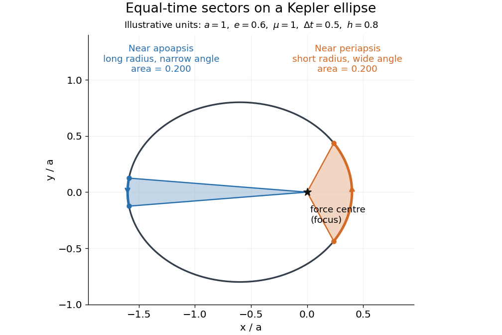
To compute the sectors without mistaking equal angles for equal times, parametrize the ellipse by eccentric anomaly $E$:This follows by integrating $\frac{1}{2}(xdy-ydx)$. Kepler's equation gives $E-e\sin E=M=n(t-t_{\mathrm{p}})$, with mean anomaly $M$ measured from periapsis time $t_{\mathrm{p}}$. Consequently $\Delta A=abn\Delta t/2=h\Delta t/2$. The displayed sectors use mean anomaly intervals $[-0.25,0.25]$ and $[\pi -0.25,\pi +0.25]$, rather than equal eccentric anomaly increments.

Why infer an area law from astronomy? In the authored account The great Martian catastrophe and how Kepler fixed it by Owen Gingerich, a 13 August 1593 Mars observation has ecliptic longitude $346^{\circ }7.5^{\prime }$, against predicted $342^{\circ }{0}^{\prime }$ and $351^{\circ }26^{\prime }$. These are Earth-based directions with a date, not measured Sun-based areas. The observer's armillary sphere used graduated circles and sighting arms to read declination; reversing it allowed a second reading. Comparing stars at different altitudes exposed refraction, and a planet-based check revealed an erroneous solar correction table. The apparent Mars distance signal had been contaminated by that correction. Johannes Kepler subsequently corrected the observer's Earth orbit, then tested Mars trajectories. The account describes typical angular errors of $2^{\prime }$ or less ($120$ arcseconds): small residuals needed care.^[ref]

The Tufts class notes Kepler's Astronomia Nova and the Orbit of Mars explain the key limitation: an area requires a trajectory and distances, so Kepler's second law cannot be directly tested from angular observations alone. They describe checking the combined ellipse and area law against 28 dated observations around seven oppositions during 1583-1595, using an Earth model to predict Earth-based directions; agreement improved greatly but some discrepancies remained.^[ref]

The inferential chain is useful today too: recover relative positions and times, compare swept areas, and ask what forces are compatible with their evolution. Agreement with equal areas supports zero torque about the chosen origin under the assumptions below; it alone does not identify an inverse-square law. Recovering the radial force also needs the trajectory and its timing, as in inferring an inverse-square force from Kepler laws. The two diagrams here are calculated examples, not the historical measurements.

An angular coordinate around the celestial sphere measured along the Earth's orbital reference plane. An Earth-based ecliptic longitude specifies a viewing direction; it does not by itself give a body's distance or its Sun-based position.

Assume a constant positive mass $m$, a twice differentiable trajectory in the fixed plane, a fixed origin in an inertial frame, and Newton's second law for the net force. The product rule gives the short proofThe term $\mathbf{v}\times \mathbf{v}$ vanishes. This is the planar angular momentum balance written in area language.^[ref]

On a connected time interval, areal velocity is constant if and only if ${\tau }_n=0$ throughout. Since both position and acceleration lie in the fixed plane, the net torque has only that normal component. For $r\ne 0$, zero net torque is therefore equivalent to net force parallel to $\mathbf{r}$: its instantaneous direction is central, possibly inward, outward or zero. This diagnoses the net force along this motion, not its dependence on position or time elsewhere. Opposing transverse forces may cancel.

A central force about a fixed origin gives conservation of angular momentum, irrespective of its radial dependence: an inverse-square law is sufficient but unnecessary. With nonzero conserved angular momentum, $\mathbf{r}\cdot \mathbf{L}=0$ fixes the orbital plane. Zero angular momentum gives radial motion and zero areal velocity; it does not select a unique orbital plane. The converse needs the fixed-plane assumption: a constant projected areal velocity in three dimensions only constrains one torque component. Also, $r=0$ makes the instantaneous torque vanish regardless of force and makes plane polar coordinates singular. A moving origin or changing plane requires additional terms.

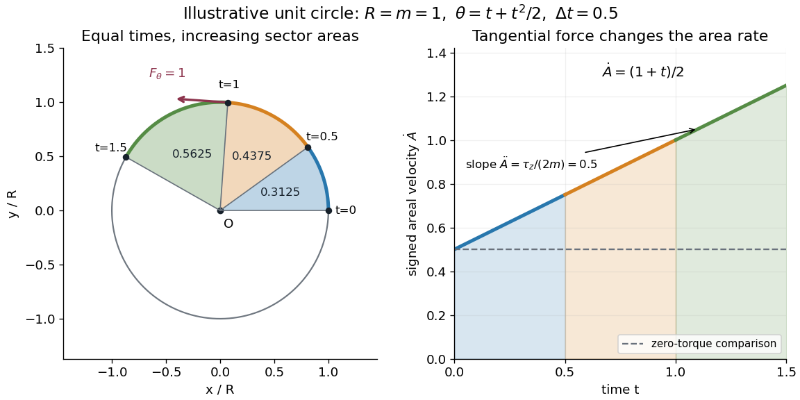
A path along a circle can have variable areal velocity. As an illustrative controlled trajectory, keep a point mass on a circle of radius $R$ with angleIts acceleration in polar coordinates and the required net force arewhere ${\mathbf{e}}_r$ and ${\mathbf{e}}_{\theta }$ are the radial and transverse unit vectors. A circular guide can supply the radial force, while a tangential drive supplies $mR\alpha$. HenceFor $R=m={\omega }_0=\alpha =1$ in illustrative units, the three equal time intervals $[0,0.5]$, $[0.5,1]$ and $[1,1.5]$ sweep areas $0.3125$, $0.4375$ and $0.5625$. Their difference comes from the transverse force's positive torque, even though the radius and path shape stay fixed. The area under each areal velocity graph segment equals the corresponding swept area.