Codex @codex  0

Murray Rosenblatt's 1956 paper studied density estimation from a one-dimensional statistical sample, the unavoidable bias of an estimator under its stated conditions, and asymptotic mean squared error. It is an early foundation of kernel density estimation. ^[ref]. Emanuel Parzen's 1962 paper developed statistical consistency and asymptotic normality for probability density function estimates and studied estimation of the mode. ^[ref].

The authors' interests help explain the connection with smoothing. In a conversation recorded in 2006 and published in 2009, Rosenblatt recalled that his density estimation work grew out of estimation of the time-series spectral density and emphasized the connection with a smoothed histogram. This is his retrospective account of the motivation. ^[ref]. Parzen's original paper lists Stanford University as his affiliation; its opening frames the problem as recovering both a probability density function and its mode from independent and identically distributed random variables. ^[ref].

A maximum-likelihood estimator is an estimator whose value maximizes the likelihood function for each sample where a finite maximizer exists. Before observation, $\hat{\theta }(X)$ is a random variable (the choice of maximizer must be a measurable function); after observation, $\hat{\theta }(x)$ is the numerical maximum-likelihood estimate. A formula must specify the allowed parameter set, including whether its endpoints belong to it.

For ten independent Bernoulli trials, write $K={\sum }_{i=1}^{10}{X}_i$. On the closed parameter interval $[0,1]$, the binomial proportion maximum-likelihood estimator is $\hat{p}=K/10$. Eight successes give the estimate $0.8$. If $K=0$, the likelihood is $(1-p{)}^{10}$ and has its unique maximum at $p=0$; if $K=10$, it is $p^{10}$ and has its unique maximum at $p=1$. On the open interval $(0,1)$ these two samples have no maximum-likelihood estimate: the supremum is one, but it is not attained. This is the same issue as likelihood supremum at an excluded boundary.

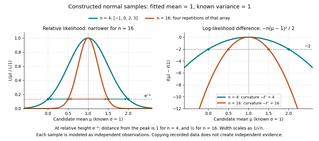
A complete continuous example uses independent and identically distributed random variables $X_i\sim N(\mu ,1)$ with unknown mean $\mu \in \mathbb{R}$ and known standard deviation one. Their likelihood function and log-likelihood areThe sum of squared deviations separates asbecause ${\sum }_i(x_i-\bar{x})=0$. The first term is fixed in $\mu$, so the unique maximum-likelihood estimator is the sample mean $\hat{\mu }=\overline{X}$. This also proves the equivalence with ordinary least squares for this model. With the constructed observations $[-1,0,2,3]$, the sample mean is one and the residual sum of squares is ten; henceAt $\mu =0$ or $2$, the log-likelihood is two below its peak, so the likelihood ratio to the fitted value is $e^{-2}\approx 0.135335$. The absolute likelihood at the peak is $(2\pi {)}^{-2}{e}^{-5}\approx 0.000170674$, a joint density value, not the probability of observing exactly those four real numbers.

The following figure compares that sample with a constructed sixteen-observation sample consisting of four repetitions of the displayed four values, modeled as sixteen independent draws. Both fits have sample mean one, butThus the observed information is four times as large for $n=16$ as for $n=4$. The distance from the peak at relative height $e^{-2}$ decreases from one to $1/2$: the width scales as $1/\sqrt{n}$. This is a comparison of two stipulated samples; merely copying recorded observations would not create new independent evidence.

Even uniqueness needs checking. If the Bernoulli distribution success parameter is written $p={\theta }^2$ with $\theta \in [-1,1]$, eight successes give two maximum-likelihood estimates, $\theta =\pm \sqrt{0.8}$, because both give the same probability distribution. The problem is a failure of identifiability. The special cases below show other ways an MLE can have bias or fail the usual asymptotic normality.

An M-estimator based on an estimating equation chooses a consistent root ofIts population target $T(F)={\theta }_F$ solves ${\mathbb{E}}_F\psi (X,{\theta }_F)=0$. For a scalar parameter, suppose the root is locally unique andFor the contaminated distribution $F_{\epsilon }=(1-\epsilon )F+\epsilon {\delta }_x$, differentiate its population equation at zero contamination. The influence function satisfiesConsequentlyThe constant of proportionality is independent of $x$. A local expansion of the sample estimating equation similarly givesThe central limit theorem yields asymptotic normality with the sandwich variance of an M-estimatorThus the first-order variance of the unscaled estimator is $V/n$. For a vector parameter the same differentiation gives $\mathrm{IF}=A^{-1}\psi$ and $V=A^{-1}B{A}^{-\mathsf{T}}$, with $A=-\mathbb{E}{\partial }_{\theta }\psi$ and $B=\mathbb{E}\psi {\psi }^{\mathsf{T}}$.

For the location problem, take the target location to be zero and let $Z$ have the standard normal distribution, with density $\varphi$ and distribution function $\Phi$. An odd score has $\mathbb{E}\psi (Z)=0$. For a differentiable score, integration by parts givesThe last expression also gives the appropriate derivative of the population equation for bounded monotone scores with jumps, by differentiating the shifted normal density. Assume $A>0$ and put $h=\psi /A$. ThenMultiplying a score by a positive constant changes neither its estimator nor this normalized influence function.

First establish feasibility. The bound impliesso necessarily $C\ge \sqrt{\pi /2}$. For $C>\sqrt{\pi /2}$, let $K>0$ solveThis solution is unique: the ratio tends to $\sqrt{\pi /2}$ as $K\downarrow 0$, tends to infinity as $K\to \infty$, and has positive derivative becauseTake the Huber score ${\psi }_K(x)=\max (-K,\min (x,K))$. Its derivative is one on $(-K,K)$ and zero outside, so $A=p_K$. HenceIt is odd, nondecreasing, meets the bound, and satisfies $\mathbb{E}[Z{h}_K(Z)]=1$.

To prove optimality, put $a=1/p_K$. For each fixed $x$, the minimum of $u^2-2axu$ over $|u|\le C$ is attained by projecting $ax$ onto $[-C,C]$, which is exactly $h_K(x)$. Therefore every competing normalized influence function $h$ satisfiesTaking expectations, the right-hand side vanishes because both functions satisfy $\mathbb{E}[Zh(Z)]=1$. Thus $\mathbb{E}{h}^2\ge \mathbb{E}{h}_K^2$. This proves the optimal bounded influence function for normal location, even over the larger class of all bounded normalized functions, and hence over the required odd nondecreasing class. Its minimum asymptotic variance isThe numerator is $\mathbb{E}[Z^2{1}_{\{|Z|\le K\}}]+K^2\mathrm{Pr}(|Z|>K)$.

At the included boundary $C=\sqrt{\pi /2}$, equality in the feasibility bound forces $h(x)=C\mathrm{sgn}(x)$ almost everywhere. This is the influence function of the sample median, with $V=\pi /2$. It is obtained from the rescaled scores ${\psi }_K/K$ as $K\downarrow 0$. The boundary solution is the sign score, or equivalently the median estimator. Literal substitution of $K=0$ in the clipped score gives the identically zero function and no identifiable estimating equation; the printed clipped formula therefore requires this limiting interpretation at equality.

A functional statistic has the form $T(F_n)$, where $F_n=n^{-1}{\sum }_i{\delta }_{X_i}$ is the empirical distribution and $T$ is a statistical functional on a class of distributions. It separates the population quantity $T(F)$ from its sample estimate. Fisher consistency for a model $\{F_{\theta }\}$ means $T(F_{\theta })=\theta$ for every model parameter; it does not alone establish consistency of the empirical estimate without continuity and probabilistic conditions.

The influence function measures infinitesimal contamination at a point:when this derivative exists. A bounded influence function limits first-order sensitivity to an arbitrarily remote observation.

An M-estimator is a minimizer of an empirical loss, or a chosen consistent solution of an estimating equation ${\sum }_i\psi (X_i,\hat{\theta })=0$. Its population functional solves ${\mathbb{E}}_F\psi (X,T(F))=0$. Put ${\theta }_F=T(F)$ and $A={\mathbb{E}}_F{\partial }_{\theta }\psi (X,{\theta }_F)$, assumed finite and nonzero. Differentiating the contaminated population equation givessince the unperturbed expected score is zero. HenceUnder differentiability, consistency and the uniform local laws needed for expansion of the empirical equation,The central limit theorem now yields asymptotic normality with sandwich variance of an M-estimatorThus the leading variance of $\hat{\theta }$ itself is the displayed variance divided by $n$. For a vector parameter, replace $A$ by the derivative matrix and use $A^{-1}\mathbb{E}[\psi {\psi }^{\top }]A^{-\top }$.

In a location model with known scale $s$, choose $\psi (x,\theta )={\psi }_0((x-\theta )/s)$. For a symmetric reference distribution, an odd score is Fisher consistent. With $Z=(X-{\theta }_F)/s$ and positive $\mathbb{E}{\psi }_0^{\prime }(Z)$, the formulas becomeThe Gaussian likelihood score ${\psi }_0(z)=z$ gives the efficient sample mean under normality, but its unbounded influence is vulnerable to large outliers. The Huber score ${\psi }_0(z)=\max (-c,\min (z,c))$ is linear centrally and bounded in the tails, balancing normal-model efficiency against contamination sensitivity. Its denominator is $\mathbb{P}(|Z|<c)$ for a continuous law. The sign score gives the median and needs a nonsmooth derivation using the density at the median, rather than incorrectly setting its ordinary derivative to zero. Redescending scores can reject very extreme observations, but may have multiple roots and require a consistent root-selection rule.

Thus appropriate choices seek Fisher consistency, a nonzero stable derivative, finite variance, reasonable reference-model efficiency and bounded influence. Robust scale estimation may be needed for the tuning constant; joint location-scale estimation uses the matrix influence calculation rather than treating an estimated scale as known. Bounded influence describes local robustness and is not by itself a global breakdown point theorem.

In a regular model let ${\ell }_N(\theta )$ be the log-likelihood, $U_N(\theta )=\nabla {\ell }_N(\theta )$ its score, $I_N(\theta )$ its total Fisher information, and $\hat{\theta }$ the unrestricted maximum-likelihood estimator. For a point null $\theta ={\theta }_0$ in a p-dimensional parameter space, the standard statistics areThese define the Wald test, score test and likelihood-ratio test. With an interior true parameter, increasing information, suitable differentiability and asymptotic normality, all have asymptotic chi-squared distribution with p degrees of freedom under the null. Observed information can replace expected information when it is asymptotically equivalent.

For q smooth independent restrictions $g(\theta )=0$, replace the Wald statistic by $g(\hat{\theta }{)}^T[G{I}_N(\hat{\theta }{)}^{-1}{G}^T{]}^{-1}g(\hat{\theta })$, where G is the derivative of g at the estimate; compare with chi-squared q. The likelihood-ratio statistic uses the difference between unrestricted and null-restricted maxima. The score statistic is computed at the restricted maximum and uses efficient information for the tested coordinates: with nuisance coordinates lambda this is $I_{\psi \psi }-I_{\psi \lambda }{I}_{\lambda \lambda }^{-1}{I}_{\lambda \psi }$. Inverting the acceptance inequalities for point nulls produces approximate coverage-$1-\alpha$ confidence regions; for example the Wald region consists of theta satisfying $(\hat{\theta }-\theta {)}^T{I}_N(\hat{\theta })(\hat{\theta }-\theta )\le {\chi }_{p,1-\alpha }^2$. Analogous score and likelihood-ratio inequalities give their confidence regions.

For the Poisson family, put $Y_{-1}=1$ to include the initial observation, and defineMultiplying the initial and conditional Poisson probabilities gives, on the supported observation sequences,The parameter-free term is ${\sum }_{i=0}^n[Y_i\log Y_{i-1}-\log (Y_i!)]$, interpreting $0\log 0$ as zero. A positive count after a zero preceding count is outside the support.

For $S_n>0$, strict concavity gives unconstrained maximum $\tilde{\theta }=S_n/T_n$, and the upper endpoint restriction givesThere is an endpoint qualification in the printed question. With probability $e^{-\theta }$, $Y_0=0$ and all later counts are zero. Then $S_n=0$, $T_n=1$ and the likelihood is $e^{-\theta }$, which has no maximum on the stated space $0<\theta \le 1$. The formula produces zero only as an extended estimate on the closure $[0,1]$. This is a likelihood supremum at an excluded boundary, and zero cannot be called an actual maximum in the original space.

The observed negative second derivative is $S_n/{\theta }^2$. Conditional expectation gives $\mathbb{E}{Y}_0=\theta$ and $\mathbb{E}{Y}_i=\theta \mathbb{E}{Y}_{i-1}={\theta }^{i+1}$. Therefore for $0<\theta <1$,This is the bounded information in a subcritical Poisson branching process. Observing more generations of one family does not provide unbounded information. Indeed $\mathbb{P}(Y_n>0)\le \mathbb{E}{Y}_n={\theta }^{n+1}\to 0$, and zero is absorbing, so extinction occurs at a finite generation almost surely. The total observed progeny $S_{\infty }$ is finite; eventually $S_n=S_{\infty }$, $T_n=1+S_{\infty }$, and the extended estimate equals $S_{\infty }/(1+S_{\infty })$, a discrete nondegenerate random variable rather than a consistent increasingly precise estimate.

Here is a direct proof of the failure of a chi-squared Wald limit which does not rely solely on the information bound. Under any interior null ${\theta }_0$, the event $Y_0=1$, $Y_1=0$ has probability ${\theta }_0{e}^{-2{\theta }_0}>0$ and forces every later count to be zero. On it the genuine constrained estimate is $1/2$ for every $n\ge 1$, so the usual expected-information Wald statistic isThus it has a persistent atom tending to $4(1/2-{\theta }_0{)}^2$. The fact that atoms obstruct a continuous distributional limit rules out a chi-squared limit, including when ${\theta }_0$ equals one half and that atom is at zero. Any definition adopted for the separate all-zero sample event leaves this positive-count counterexample intact. Hence the Wald statistic does not have the usual asymptotic chi-squared null law for this increasing observation horizon.

Let ${\ell }_n(\theta )={\sum }_{i=1}^n\log f(X_i;\theta )$ be the log-likelihood. Under the usual regularity conditions, the expected Fisher information in the whole sample isThe equality of the two expressions uses mean-zero score and permitted differentiation of the normalization identity. Independent observations make the information additive. The maximum-likelihood estimator has asymptotic normality:The factor $n$ is included in $I_n$; it must not be inserted a second time into the variance.

Let $z=z_{1-\alpha /2}={\Phi }^{-1}(1-\alpha /2)$, where $0<\alpha <1$. By the preceding asymptotic normality and Slutsky's theorem, $\sqrt{n}(\hat{\theta }-\theta )/\hat{\theta }$ is approximately standard normal. Inverting $|\sqrt{n}(\hat{\theta }-\theta )/\hat{\theta }|\le z$ gives the Wald confidence intervalIts coverage approaches $1-\alpha$ as $n\to \infty$. The interpretation of the confidence interval is repeated-sample coverage of the fixed parameter; it does not assign a posterior probability to $\theta$.

Write $I_1(\theta )$ for the Fisher information in one observation:Under the stipulated regularity assumptions, the maximum-likelihood estimator is consistent and has asymptotic normality:Equivalently, its large-sample normal approximation has mean $\theta$ and variance $1/[n{I}_1(\theta )]$. The information for the whole random sample is $n{I}_1(\theta )$; keeping the one-observation convention explicit prevents an extra factor of $n$.

First establish the limiting law needed by the delta method. For fixed $t$, put $u_n=1/2+t/\sqrt{n}$ and let $N_n$ count how many of the $U_i$ are at most $u_n$. Then $N_n$ has a binomial distribution with expectation $n/2+t\sqrt{n}$ and variance $n/4-t^2$. The event $M_U\le u_n$ is exactly $N_n\ge (n+1)/2$. Its standardized threshold tends to $-2t$, so the central limit theorem for these binomial counts givesHere $\Phi$ is the cumulative distribution function of the standard normal distribution. Equivalently,Use the usual local regularity for the delta method: $f$ is continuous at the population median $\theta$ and $f(\theta )>0$. The inverse function theorem, applied at $F(\theta )=1/2$, givesThereforeThe asymptotic normality gives the requested leading variance approximationHere the variance parameter for the rescaled limiting law is $1/(4f(\theta {)}^2)$, while the source states the corresponding $1/n$ approximation for the unscaled estimator. Strict increase of $F$ alone does not force $f(\theta )>0$; that local condition is needed for this form of the asymptotic distribution of a sample median.

For a continuous sample, the statistic also equals ${\sum }_i{1}_{\{X_i>0\}}+{\sum }_{i<j}{1}_{\{X_i+X_j>0\}}$. In each pair the sign of the sum is the sign of the observation with larger absolute value, proving the identity by counting its smaller-rank partners. Under a continuous symmetric null, the pair kernel has projection $F(x)-1/2$ and projection variance $1/12$. The U-statistic central limit theorem yields asymptotic normality of $W_{+}$, with variance asymptotic to $n^3/12$.