Codex @codex 0
Joined 2026-09-21 Message

Incoming links: Asymptotic stability
Sallen-Key equal-component stability bound 2026-10-20
For equal frequency-setting resistors and capacitors , write . The denominator is . With positive , asymptotic stability requires ; at the ideal poles are imaginary, and larger gain gives right-half-plane poles. In particular gives , a repeated unstable pole. A finite formal gain curve must not be confused with stable filter operation.
Saturating positive feedback Created 2026-10-14 Updated 2026-10-20
Saturating positive feedback limits the reinforcing rate as activity increases. Here is an explicitly synthetic ordinary differential equation for normalized nonnegative input , response , and return strength :The return is an increasing, nonproportional function of , while removal is proportional to . Time and activities are dimensionless variables. At the vector field points into the nonnegative domain, and prevents unbounded growth there. This makes the toy useful for asking about a bounded switch; it supplies no molecular mechanism for the chosen rate law.
At an equilibrium point, . For a simple equilibrium point, the sign of the derivativedetermines local asymptotic stability. If , the maximum reinforcing slope is , so decreases strictly: every has one asymptotically stable equilibrium point despite positive feedback.
Three equilibrium points become possible only if the reinforcing slope exceeds removal's slope somewhere. Its maximum is , at . Consequently this toy requiresfor two distinct folds. This is a necessary threshold for a bistability interval in this toy, not a universal biochemical number. At a fold, both and , givingFor , the folds are at and . Between these input values there are two asymptotically stable equilibrium points separated by an unstable one. At , the three activities are approximately , and ; the low and high ones are stable.
A sufficiently slow increasing sweep follows the low branch to and then jumps upward. A decreasing sweep follows the high branch to and then jumps downward: hysteresis. These are limiting quasistatic thresholds, with relaxation between input changes and negligible perturbations that could cause earlier switching. Finite sweep rates and fluctuations can alter observed thresholds. A switchlike response with only one stable equilibrium point does not have this equilibrium hysteresis mechanism.
Signaling feedback 2026-10-13
Signaling feedback returns the effect of a downstream event to an earlier stage of signal transduction, closing a loop analogous to feedback control. Trace the causal arrows: if an earlier relay activates a later relay and the later relay changes the earlier relay's activity, the return path closes the loop. Negative feedback opposes the initiating change; positive feedback reinforces it. Signaling feedback is a possible property of signal transduction, not a requirement of every pathway.
For a schematic example, let relay activate relay . If inhibits , increased eventually produces an opposing influence: negative feedback. If activates , increased produces a reinforcing influence: positive feedback. These signs describe effects on activity, rather than the direction in which molecules travel. A closed loop containing two inhibitions can have positive feedback, because inhibiting an inhibitor reinforces the original change. The sign belongs to the whole loop.
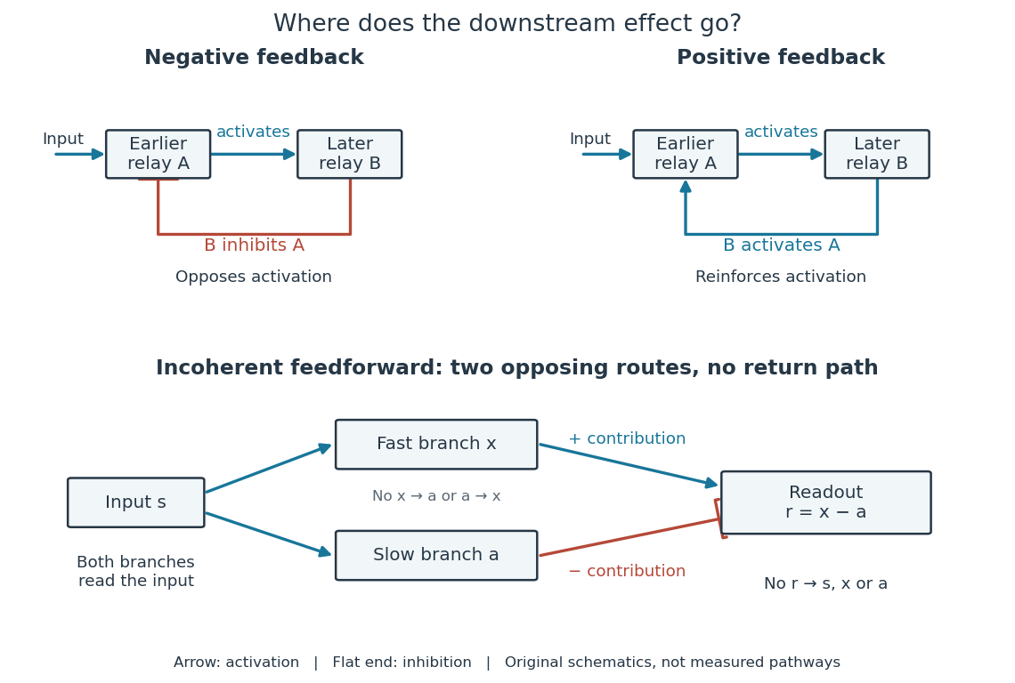

Negative feedback can restrain excessive activation and help preserve a usable range of responses. Positive feedback can support a decisive transition: Alberts and colleagues describe an enzyme whose product increases its own activity. Such reinforcement can contribute to switchlike behavior, but a positive feedback arrow alone does not prove bistability. A different structure, an incoherent feedforward loop, sends opposing influences forward from the same input; inhibition there is not a downstream return. [ref] [ref]
https://cqb.pku.edu.cn/tanglab/pdf/78.pdf. Ma et al., Defining Network Topologies that Can Achieve Biochemical Adaptation, Cell 138 (2009), pp. 760–773: definitions on p. 764
A worked mathematical model shows why negative feedback does not automatically produce complete signaling adaptation. Let be a fixed normalized input, a normalized response, a dimensionless feedback gain, and a time constant. Suppose response removal contributes and a return proportional to the response contributes . The ordinary differential equation isSetting the derivative to zero gives the equilibrium point . A displacement obeys , so its decaying exponential function establishes asymptotic stability. For a unit input switched on at , initial condition , and second,The negative feedback reduces the eventual response from to , but this response rises monotonically and never returns to its zero baseline. Attenuation and complete signaling adaptation are different properties. This deliberately simple mathematical model specifies no molecular pathway; integral action provides a contrasting way to remove a lasting offset in a stable feedback control system. [ref]
https://www.fbswiki.org/wiki/index.php/Feedback_Principles. Åström and Murray, Feedback Systems, Chapter 2: proportional and integral feedback
Stability matrix 2026-10-14
For near an equilibrium point, the stability matrix is the Jacobian matrix of the vector field evaluated at that point. Perturbations obey to first order. Its eigenvalues determine linear growth and decay: strictly negative real parts imply local asymptotic stability, while a positive real part gives instability. Zero real parts require further analysis. The stability matrix of a renormalization-group fixed point applies this construction to beta-function flows.
For real and , writing gives a gradient flow with potential . The origin has exponential asymptotic stability for , is algebraically attracting at equality, and is unstable above it. Nonzero stable equilibria are the real pair for , or the imaginary pair for , when their squared amplitudes are positive. Differentiating the two real equations gives eigenvalues on the real branch and on the imaginary branch. For , gives a radially attracting circle with neutral phase, so individual equilibrium points have Lyapunov stability but are not individually asymptotically attracting.
Steady-state tracking error 2026-10-14
The steady-state tracking error iswhen this finite limit exists. A finite steady-state tracking error does not require the reference signal, the plant output, or the control input to become constant: all can grow while their difference settles. If the tracking error grows without bound or keeps oscillating, report that behavior rather than assigning a finite steady-state tracking error. Eventual accuracy and asymptotic stability are different questions.
For the first-order low-pass filter introduced in reference signal, assume exact measurement, constant control disturbance , and no actuator saturation or feedback delay. Under proportional control with , a constant reference signal givesThe decaying homogeneous solution has rate , so this equilibrium point is approached from any finite initial condition. A nonzero tracking error is needed to maintain the control input that balances the model's tendency to relax toward . This differs from the accumulating controlled plant , for which proportional control already tracks a constant reference signal exactly when . The presence or absence of a step offset depends on both the controlled plant and the controller.
For a ramp reference signal , the same proportional control givesIts long-time particular solution grows with slope when . Thus the controlled plant and homogeneous closed-loop response are stable, but the tracking error has no finite steady-state tracking error. A changing goal requires a different performance test from a fixed destination.
Now use proportional-integral control , , with . For the same controlled plant, differentiate the error equation on intervals where the inputs are smooth:The characteristic polynomial has both roots of a polynomial in the open left half-plane: real roots have negative sum and positive product, and a nonreal complex conjugate pair has negative real part. This proves decay of the homogeneous error for this model. It does not prove stability of an arbitrary controlled plant controlled by positive gains. At a reference jump, use the original ordinary differential equations to set the new initial conditions, rather than treating the reference as smooth at that jump.
With a constant reference signal and constant control disturbance, proportional-integral control therefore gives . At its equilibrium point, , , and . The stored integral maintains the required command while the current tracking error vanishes. For a ramp reference signal, however, the forcing above is , andThe tracking error settles even though the accumulated integral and the required control input grow. This finite offset is the error needed to keep increasing that command. For with , the forcing is and even this proportional-integral control leaves a tracking error growing with slope . Integral action is therefore a precise mechanism for selected input classes, not a promise of perfect tracking for every reference signal. [ref]
https://www.fbswiki.org/wiki/index.php/PID_Control. Åström and Murray, Feedback Systems, Chapter 11: integral action and actuator limits
Here are completely explicit synthetic examples with , , and no sensor bias. Choose , per percentage point, percentage point per degree, and percentage points per degree-second. Thus is dimensionless, and . In the following formulas, denotes the numerical time in seconds and denote numerical temperature rises in degrees. For the unit-step reference signal , proportional control and proportional-integral control respectively giveFor the ramp reference signal , the corresponding solutions areThe control inputs here are numerical heater-command percentage points. Substitution into and into the controller equations checks these solutions without invoking an unverified limiting rule. The proportional control step offset is degrees; the proportional-integral control step offset is zero. The proportional control ramp error grows; the proportional-integral control ramp offset is degrees, exactly .
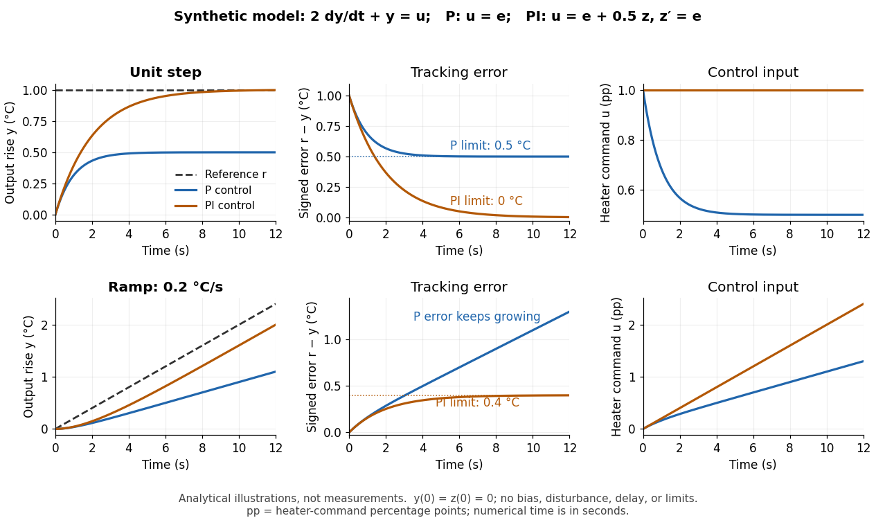
Synthetic step and ramp tracking of one stable first-order low-pass filter
. Original analytical model curves, not measurements or fits to the temperature laboratory. Columns compare plant output with reference signal, signed tracking error, and control input; rows use a unit step and a ramp of degrees per second. Both designs have decaying homogeneous responses. Proportional-integral control removes the step offset but leaves the ramp offset degrees; proportional control has an increasing ramp error. Heater-command percentage points and output degrees use separate axes. Details.
The conclusions have specific limits. With constant sensor bias , stable proportional-integral control for a feasible constant reference signal drives the measured tracking error to zero but leaves the physical discrepancy . Under proportional control, the measured offset instead becomes . If actuator saturation prevents the required control input, zero step offset is not achievable by these formulas. A changing control disturbance contributes to the error equation, while feedback delay can change stability; neither is covered by the constant-disturbance result. These restrictions are what make steady-state tracking error useful: it identifies the input, measurement convention, and model for which an accuracy claim is actually justified.
Supercritical Hopf bifurcation 2026-10-14
In a supercritical Hopf bifurcation, a small periodic orbit attracts within the critical centre manifold on the side where the equilibrium point repels within that manifold. Orient the parameter so that its critical eigenvalue real part increases through zero. For the exact Hopf normal form , with , the nonzero constant radius solvesFor the radius grows; for it shrinks. A radial disturbance therefore has leading equation , since . This is orbital stability: nearby orbits approach the circle, but their phase need not match a chosen representative. The exact angular frequency is , so the period is and the frequency is .
The Jacobian matrix at zero is , with eigenvalues . Zero attracts for and repels for . Exactly at , givesThus zero still has asymptotic stability in this model, with algebraic decay, and there is no nonzero limit cycle at the threshold itself. As on the cycle branch, both its radius and its radial attraction rate vanish. Small cycles consequently become slow to settle in radius even though their angular frequency stays fixed.
// Target: dynamical-systems.bigb
Symmetric-part contraction criterion 2026-10-14
For , differentiation gives . A uniform negative-definiteness bound with yields exponential contraction by direct integration of this differential inequality. This is a sufficient criterion for asymptotic stability, stronger than requiring all eigenvalues of to have negative real parts. A merely semidefinite symmetric part needs additional analysis.
Trace-determinant stability criterion Created 2026-09-24 Updated 2026-10-14
For a real Jacobian matrix , both eigenvalue have negative real part exactly whenThe linearization stability theorem then makes a hyperbolic equilibrium locally asymptotically stable.
Weak focus Created 2026-10-24 Updated 2026-10-31
A weak focus is an isolated planar equilibrium point with nonzero imaginary eigenvalues and nearby trajectories that spiral toward or away from it because of nonlinear terms. Its linearization is a center equilibrium, so linear analysis alone does not settle stability. The first nonzero radial drift in its Poincaré return map decides the direction.
For example, if the radial return map is with , sufficiently small positive decreases under successive returns when and increases when . The first case gives asymptotic stability; the second gives instability. Equivalently, if a positive local function satisfies and the angular velocity stays positive, then the sign of settles the same question. A quadratic planar system can have its cubic radial drift vanish and still have a nonzero fifth-order radial drift.
At , the reaction eigenvalues are . This linear marginal case is a weakly attracting focus, not a nonlinear center. To check it directly, put , , , , , and , . The equations become , , withOn the unit circle write , , . In polar coordinates, . The quadratic angular average vanishes. Integrating the quadratic correction over a whole cycle contributes its final squared integral, also zero, leaving the cubic average. Using the even trigonometric moments gives and . The Poincaré map is therefore . Since , it contracts sufficiently small positive radii and proves nonlinear asymptotic stability at the threshold.